Analytic Solutions to Optimal Control Problems with Constraints

(1)

http://dx.doi.org/10.4236/am.2015.614205

Analytic Solutions to Optimal Control

Problems with Constraints

Dan Wu

Department of Mathematics, Henan University of Science and Technology, Luoyang, China

Received 25 November 2015; accepted 28 December 2015; published 31 December 2015

This work is licensed under the Creative Commons Attribution International License (CC BY). http://creativecommons.org/licenses/by/4.0/

Abstract

In this paper, the analytic solutions to constrained optimal control problems are considered. A novel approach based on canonical duality theory is developed to derive the analytic solution of this problem by reformulating a constrained optimal control problem into a global optimization problem. A differential flow is presented to deduce some optimality conditions for solving global optimizations, which can be considered as an extension and a supplement of the previous results in canonical duality theory. Some examples are given to illustrate the applicability of our results.

Keywords

Constrained Optimal Control, Analytic Solution, Canonical Duality Theory, Global Optimization

1. Introduction

In this paper, we consider the following linear-quadratic optimal control problem involving control constraints:

( )

( ) ( )

( )

0

T T

0 0 0

1

min , d

2

. . , , , , ,

f

t

f

J x u x t Qx t u t Ru t t

s t x t Ax t Bu t x t x u t U t t t

= +

 

= + = ∈ _{∈ } _

∫



 (1)

where Q∈n n× is a positive semidefinite symmetric matrix, R∈m m× is a positive definite symmetric ma-trix, and A∈n n× , B∈n m× are two given matrices. x t

( )

∈n is a state vector, and u t

( )

∈m is an ad-missible control taking values on the set U, which is integrable or piecewise continuous on _t t₀, _f_. In our work, we suppose that U is a closed convex set, and we study two forms of the set U, a sphere constraint and box con-straints respectively. Problems of the above type arise naturally in system science and engineering with wide applications [1][2].

(2)

In the unconstrained case, an optimal feedback control can be successfully obtained which seems to be a perfect result. For constrained optimal control problems the level of research is less complete. It is now well known that common approaches are based on applying a quasi-Newton or sequential quadratic programming (SQP) tech-nique to the constrained; see for instance [4]-[8] and the references therein. But due to the presence of state or control constraints, all the above methods are trapped in analytical difficulties and thus are not guaranteed to find analytic solutions to the constrained, at best, they can provide numerical solutions.

In this paper, a different way, canonical dual approach is used to study the problem

( )

 by converting the original control problem into a global optimization problem. The canonical duality theory was developed from nonconvex analysis and mechanics during the last decade (see [9][10]), and has shown its potential for global optimization and nonconvex nonsmooth analysis [10]-[14]. Meanwhile, we introduce a differential flow for constructing the so-called canonical dual function to deduce some optimality conditions for solving global opti-mizations, which is shown to extend some corresponding results in canonical duality theory [9]-[11]. In com-parison to the previous work mainly focused on simple constraints, we not only discuss linear box constraints, but also the nonlinear sphere constraint. Then combining the canonical dual approach given in this paper with the Pontryagin maximum principle, we solve the constrained optimal control problem

( )

 and characterize the analytic solution expressed by the co-state via canonical dual variables.

Now, we shall give the Pontryagin maximum principle and an important Lemma.

Pontryagin Maximum Principle If uˆ

( )

⋅ is an optimal solution to the problem

( )

 and the corresponding

state and co-state are denoted by xˆ

( )

⋅ and

λ

ˆ

( )

⋅ respectively, for the Hamilton function

(

_ˆ

)

_ˆT

(

)

1 T 1 T

, , , ,

2 2

H t x u

λ

=

λ

Ax+Bu + x Qx+ u Ru (2) then we have,

(

ˆ

)

( )

0 0

ˆ , , ,ˆ ˆ ˆ ˆ, ˆ ,

x=H_λ t x u

λ

=Ax+Bu x t =x (3)

(

)

T

( )

ˆ _{, , ,}_{ˆ ˆ} ˆ ˆ _ˆ_, ˆ _0,

x f

H t x u A Qx t

λ= − λ = − λ− λ = (4) and

( ) ( ) ( )

(

,ˆ ,ˆ ,ˆ

)

min

(

,ˆ

( ) ( ) ( )

, ,ˆ

)

, a.e. 0, f . u U

H t x t u t λ t H t x t u t λ t t t t

∈  

= _{∈ } _ (5)

Lemma 1. An admissible pair

(

x t u tˆ

( ) ( )

,ˆ

)

is an optimal pair to the primal problem

( )

 if and only if this pair

(

x t u tˆ

( ) ( )

,ˆ

)

satisfies the Pontryagin maximum principle (3), (4) and (5).

Proof. Denote

(

, ,ˆ

)

min

(

, , ,ˆ

)

a.e. 0, f . u U

H∗ t xλ H t x u λ t t t

∈  

= _{∈ } _ (6) Let

(

x t u t

( ) ( )

,

)

be an arbitrary admissible pair satisfying (3). By the definition of H∗, we have

(

_{, ,} ˆ

) (

_{, , ,} ˆ

)

H∗ t x

λ

≤H t x u

λ

, and H∗

(

t x, ,

λ

ˆ

)

is equivalent to the following global optimization

( )

T T

0

1 _ˆ

min , a.e. , .

2 f

u U∈ u Ru λ t Bu t t t

 

+ _{∈ } _ (7)

Moreover, it is easy to see that the minimizer uˆ of (7) depends only on the co-state λˆ, i.e. uˆ 0

x

∂ =

∂ , which implies that

(

_ˆ

)

(

_ˆ

)

(

_ˆ

)

ˆ

(

_ˆ

)

ˆ ˆ ˆ

, , , , , , , , , , , .

x x u x

u

H t x H t x u H t x u H t x u

x

λ λ λ λ

∗ ₌ ₊ ∂ ₌

∂ (8) Taking into account of the convexity of the integrand in the cost functional as well as the set U, the function

(

_{, ,}ˆ

)

H∗ t xλ is convex in x, and

(

)

(

)

(

)

(

)

(

)

(

)

(

)

T

ˆ _ˆ ˆ _ˆ ˆ _ˆ

, , , , , ,

ˆ ˆ

ˆ ˆ ˆ ˆ ˆ

, , , , , , ,

x

H t x H t x H t x x x

H t x u H t x u x x

λ λ λ

λ λ

∗ _≥ ∗ ₊ ∗ ₋

(3)

which leads to

(

_{ˆ ˆ} _ˆ

) (

_ˆ

)

_ˆT

(

_ˆ

)

, , , , , , .

H t x u λ −H t x u λ ≤λ x−x

Thus, we have

( )

( ) ( ) ( )

(

)

(

( ) ( ) ( )

)

( ) ( ) ( )

(

)

( ) ( ) ( )

(

)

( ) ( ) ( )

(

)

T

0 0

0

T T

0 0 0

ˆ

ˆ ˆ ˆ

, , , , , , d d

ˆ _ˆ ˆ _ˆ

d 0.

f f

f

t t

J u J u

H t x t u t t H t x t u t t t t x t x t t

t x t x t t x t x t

λ λ λ

λ λ

⋅ − ⋅        

 

= _ − _ + −

 

≤ _ − _= − − =

∫



 (9)

This means that J attains its minimum at uˆ. The proof is completed.

The above Lemma reformulates the optimal control problem

( )

 into a global optimization problem (7). Based on this fact, we can derive the analytic solution of the problem

( )

 by only solving problem (7) via the canonical dual approach.

The rest of the paper is organized as follows. In Section 2, we consider the optimal control problem with a sphere constraint. By introducing the differential flow and canonical dual function for solving global optimiza-tions, we derive the analytic solution expressed by the co-state via canonical dual variables. Based on the similar canonical dual strategy, the box constrained optimal control problem is studied and the corresponding analytic expression of optimal control is obtained in Section 3. Meanwhile, some examples are given to demonstration.

2. Sphere Constrained Optimal Control Problem

In this section, we let

( )

1 T

( ) ( )

, 0 2

m

U=u t ∈ u t u t ≤a a> 

   be a sphere. Before we go to derive the analytic

solution for the problem

( )

 , we first make some preliminary concepts and theorems in solving global optimi-zation over a sphere based on canonical duality theory which will be used in the sequel.

2.1. Global Optimization over a Sphere

Consider the following general optimization problem

( )

1 T

min . . , ,

2

P u s t u∈U U=_ u u≤a_

  (10) where P u

( )

is assumed to be twice continuously differentiable in _m_.

The original idea of this section is from the paper [13] by Zhu. Denote

( )

{

2

}

0, 0, for every .

P u I u U

ρ  ρ  ρ

= ∈ _∇ + _> ≥ ∈

 

 is an open set with respect to

[

0,+∞

)

, and it is easy to see that if ρ ∈ˆ , then

ρ

∈ for any ρ ρ≥ ˆ. Assume that a ρ∗∈ and a nonzero vector u∗∈U such that

( )

0.

P u∗ ρ∗ ∗u

∇ + = (11) We focus on the differential flow uˆ

( )

ρ which is well defined near ρ∗ by

( )

1

2

ˆ d

ˆ ˆ 0,

d

u

P u ρI u

ρ

−

 

+ ∇_ + _ = (12)

( )

ˆ .

(4)

( )

(

( )

)

T

( ) ( )

ˆ ˆ ˆ ,

2

d

P

ρ

=P u

ρ

+

ρ

u

ρ

u

ρ

−

ρ

a (14) and the canonical dual problem associated with the problem (10) can be proposed as follows

( )

(

( )

)

T

( ) ( )

ˆ ˆ ˆ

: max .

2

d d

P P ρ =P u ρ +ρu ρ u ρ −ρ ρa ∈ 

  (15)

Notice that

( )

(

( )

)

( )

2

1

T 2

2 d

ˆ ˆ ˆ

d

P

u P u I u

ρ _ρ _ρ _ρ _ρ

ρ

−

 

= − _∇ + _ . By the definition of , it follows that the canonical dual function Pd

( )

ρ

is concave on . For a critical point ρ ∈ˆ , it must be a global maximizer of Pd

( )

ρ

on , sometimes, which leads to a global minimizer uˆ=uˆ

( )

ρ

ˆ of (10).

Theorem 1. If the flow uˆ

( )

ρ (defined by (11)-(13)) meets a boundary point of the ball U at ρ ∈ˆ  such that 1ˆT

( ) ( )

ˆ ˆ ˆ ,

2u

ρ

u

ρ

=a then uˆ

( )

ρˆ is a global minimizer of P u

( )

over U. Further one has

( )

(

( )

)

( )

ˆ

ˆ ˆ

ˆ

min d max d .

u U∈ P u =P u ρ =P ρ = ρ ρ≥ P ρ

(16) Detailed proof of Theorem 1 can be referred to [13]-[15].

In what follows, we show that uˆ

( )

ρ can be derived by solving backward differential equation.

Lemma 2.Let uˆ

( )

ρ

be a given flow defined by (11)-(13). We call uˆ

( )

ρ

, ρ∈

(

0,ρ∗_ a backward diffe-rential flow.

Since U is bounded and P u

( )

is twice continuously differentiable, we can choose a large positive parameter ρ∗_{such that}_∇2_{P u}

( )

₊ρ∗_I_>₀

  , ∀ ∈u U and

ρ

supU

{

P u

( )

}

∗_> _∇

. If ∇P

( )

0 ≠0, then it follows from

( )

2

1

P u

ρ

∗

∇

< uniformly in U that there is a unique nonzero fixed point u∗∈U such that

( )

P u

u

ρ

∗ ∗ ∗ −∇

= (17) by Brown fixed-point theorem, which means that the pair

(

u∗,ρ∗

)

satisfies (11). Then we can solve (11) backwards from

ρ

∗ to get the backward flow uˆ

( )

ρ

, ρ∈

(

0,ρ∗_. We refer the interested reader to [16][17]

for detail of choosing the desired parameter

ρ

∗.

2.2. Analytic Solution to the Sphere Constrained Optimal Control Problem

Let

( )

1 T ˆT

( )

2

P u = u Ru+

λ

t Bu in (10). Based on the canonical dual approach in Section 2.1, a relationship between u∈m and ρ∈ =

[

0,+∞

)

(since R is a positive definite matrix) is well defined as

( )

[

]

1 T

( )

0 ˆ

ˆ a.e. , f .

u

ρ

= − R+

ρ

I − B

λ

t t∈ t t _ (18) So, the canonical dual function can be formulated as, for each

ρ

≥0

( )

1 ˆT

( ) (

)

1 T_ˆ

( )

. 2

d

P

ρ

= −

λ

t B R+

ρ

I − B

λ

t −a

ρ

(19) Next, we have the following properties.

Lemma 3. Let uˆ

( )

ρ be a given flow defined by (18) and

( )

1 _ˆT

( ) ( )

_ˆ

2

y ρ = u ρ u ρ , we have

( )

T

_{( ) ( )}

_{( )}

d 1

ˆ ˆ ,

d 2

d

P

u u a y a

ρ

ρ ρ ρ

(5)

( )

_{( ) [}

T

_{] ( )}

ˆ ˆ

d d d

.

d d d

y u u

R I

ρ

  = −  +

  (21)

Proof. Since Pd

( )

ρ

is differentiable,

( )

_{( )}

(

)

_{( )}

( ) (

) (

)

( )

( ) ( )

1

T T

1 1

T T

T

d

d _{1 ˆ} _ˆ

d 2 d

d

1 ˆ ˆ

2 d

1

ˆ ˆ .

2

d _R _I

P

t B B t a

R I

t B R I R I B t a

u u a

ρ ρ

λ λ

ρ ρ

ρ

λ ρ ρ λ

ρ ρ ρ

−

− −

 ₊   

= − −

+

= + + −

= −

( )

_{( ) ( )}

_{( ) [}

T

_{] ( )}

T ˆ ˆ ˆ

d d d d

ˆ .

d d d d

y u u u

u R I

ρ

  = = −_ _ +

 

( )

ρ

be a given flow defined by (18), and Pd

( )

ρ

be the corresponding canonical dual

function defined by (19).

1) y

( )

ρ is monotonously decreasing on

[

0,+∞

)

.

2) if there exists ρˆ∈

[

0,+∞

)

such that uˆ

( )

ρˆ ∈U, then Pd

( )

ρ

is monotonously decreasing on

[

ρˆ ,+∞

)

.

Proof. By (21), it follows that d

( )

0

d

y ρ

ρ ≤ for any

ρ

∈

[

0,+∞

)

, which means that y

( )

ρ

is monotonously

decreasing on

[

0,+∞

)

.

If there exists one point

ρ

ˆ∈

[

0,+∞

)

and uˆ

( )

ρ

ˆ ∈U such that y

( )

ρ

ˆ ≤a, by the monotonous decline of

( )

y

ρ

, we have uˆ

( )

ρ

∈U for any ρ ρ≥ ˆ. By (20), we can conclude that Pd

( )

ρ

is monotonously decreas-ing on

[

ρ

ˆ,+∞

)

. The proof is completed.

Theorem 2. For the sphere constrained optimal control problem

( )

 , the analytic solution expressed by the

co-state is given as follows

( )

1

T

ˆ ˆ

ˆ opt ,

u R ρ λ I B λ

−

 

= −_ + _ (22)

where

ρ

opt

( )

λ

ˆ with respect to the co-state λˆ is defined by the following condition

( )

T 2 T T 2 T

ˆ ˆ ˆ

ˆ if 2 ,

ˆ

ˆ ˆ

0 if 2 ,

opt BR B a

BR B a

ρ λ λ λ ρ λ

λ λ

−

 _>

 = 

 ≤



(23)

and

ρ λ

ˆ

( )

ˆ satisfies the equation

( )

2

T T

ˆ _{B R} ˆ _I _B ˆ _{2 ,}_a ˆ _0.

λ  ₊ρ λ − λ₌ ρ λ _≥

 

Proof. We first consider BT

λ

ˆ

( )

t ≠0 for some one point t∈ t t₀, _f_.

For any ρ∈

[

0,+∞

)

, when BT

λ

ˆ

( )

t ≠0, with (12), (18) and taking into account of Lemma 3, we have

( )

ˆ 0

u ρ ≠ and dˆ

( )

0 d

u ρ

ρ ≠ . This means that y

( )

ρ is strictly monotonously decreasing on

[

0,+∞

)

.

Case 1: Suppose that 1_ˆT

( ) ( )

₀ _ˆ ₀

2u u >a. Since y

( )

ρ

is continuous and strictly monotonously decreasing on

[

0,+∞

)

and y

( )

ρ

→0 as ρ → +∞, there must exist one point ρ >ˆ 0 such that 1ˆT

( ) ( )

ˆ ˆ ˆ

2u ρ u ρ =a, i.e.

( )

ˆ ˆ

u

ρ

∈U, which leads to uˆ

( )

ρ

∈U for any ρ ρ≥ ˆ. For each element ρ ρ ρ, ≥ ˆ, the function f_ρ

( )

u is given as follows

( )

1 T 1 T _ˆT

( )

1 T

,

2 2 2

f_ρ u =P u +ρ_ u u−a_= u Ru+λ t Bu+ρ_ u u−a_

(6)

where ρ is a parameter. It is obvious that P u

( )

≥ fρ

( )

u for all u∈U. Since fρ

( )

u is twice continuously differentiable in m, there exists a closed convex region  containing U such that on , ∇2f_ρ

( )

u >0 and

( )

(

ˆ

)

0

f_ρ u ρ

∇ = . This implies that uˆ

( )

ρ is the unique global minimizer of f_ρ

( )

u over . By (18) and (19), we have

( )

(

)

1 ˆT

( )

[

]

1 T_ˆ

( )

ˆ ,

2

d

fρ u

ρ

= −

λ

t B R+

ρ

I − B

λ

t −

ρ

a=P

ρ

and

( )

min

( )

(

ˆ

( )

)

d

( )

.

u U

P u f_ρ u f_ρ u f_ρ u

ρ

P

ρ

∈

≥ ≥ = = (25)

Further, it follows from Lemma 4 that

( )

(

( )

)

ˆ ˆ ˆ ˆ

maxPd Pd P u .

ρ ρ≥ ρ = ρ = ρ (26) Thus, for every u∈U, when ρ ρ≥ ˆ, we have

( )

( ) ( )

( )

T T T T

ˆ

1 _ˆ 1 _ˆ

ˆ ˆ ˆ ˆ

ˆ ˆ ˆ

min max .

2 2

d d

u U∈ u Ru+

λ

t Bu= u

ρ

Ru

ρ

+

λ

t Bu

ρ

=P

ρ

= ρ ρ≥ P

ρ

Case 2: Suppose that 1ˆT

( ) ( )

0 ˆ 0

2u u ≤a. It is easy to verify that

( ) ( )

T

1

ˆ ˆ

2u

ρ

u

ρ

<a for any

ρ

>0, and

( )

0

maxPd Pd 0

ρ≥ ρ = . Then, by using the similar proving strategy in case 1, we can show that uˆ 0

( )

is a global minimizer of (7) in case 2.

On the other hand, If there exists one point t∈ t t₀, _f_ such that BT

λ

ˆ

( )

t =0, then (7) is equivalent to the problem min1 T

2

u U∈ u Ru, and it is clear that uˆ 0

( )

=0 is a global minimizer of this problem.

Define

( )

ˆ if ˆ 0 2 , ˆ

0 if 0 2 ,

opt u a

u a

ρ

ρ _{= } >

≤ 

where ρˆ is the only solution of the equation

[

]

1 T_ˆ

( )

[

)

2 , 0,

R+ρI − B λ t = a ρ∈ +∞ under the condition

( )

ˆ 0 2

u > a. Based on canonical duality theory, ˆ

( )

opt

u ρ is a global minimizer of the problem (7). Hence, by Lemma 1, we can derive the optimal solution

( )

1 _T

( )

0 ˆ

ˆ opt opt , a.e. , f .

u

ρ

= −_R+

ρ

I_− B

λ

t t∈ t t _ (27) If consider ρopt_{as a function with respect to the co-state} λ_ˆ_{, we can define the function} ρopt

( )

λ_ˆ

satisfy-ing (23), and the analytic solution by the co-state to the problem

( )

 can be given as (22). This completes the proof.

Theorem 3. Let R be an identity matrix I in (1). Then the analytic solution to problem

( )

 is obtained as

follows

T

T ˆ

ˆ .

ˆ max 1,

2

B u

B a

λ λ = −

       

(28)

Proof. Suppose that R=I. By Theorem 2, it follows that

( )

T_ˆ

max 0, 1 2

opt B t

a

λ ρ =  − + 

 

 

(7)

solution can be expressed as, a.e. t∈ t t₀, _f_,

( )

T 1

T

ˆ ˆ

ˆ .

ˆ max 1,

2

opt opt B t

u R I B t

B t

a

λ

ρ ρ λ

λ

−

 

= −_ + _ = −

 

 

 

This concludes the proof of Theorem 3.

2.3. Applications

Now, we give an example to illustrate the applicability of Theorem 2. We consider the following sphere con-strained optimal control problem.

Example 1: In (1), we consider

3 1 2

5 0 7

4 4.5 7

A

−

 

 

= −_ _

 ₋ 

 

,

3.5 2

2 6

8 9

B

−

 

 

=  

 ₋ 

 

,

2 5 7

1 2 1.5

3 0 8

Q

− −

 

 

=  

₋ 

 

, R=I_{2 2}× ,

( ) (

)

T

0 1, 1, 1

x = − − − , t₀=0, t_f =1, and 1 2

a= . Q≥0 and R>0 satisfy the assumptions in this paper. By Lemma 1 and Theorem 2, in order to derive the optimal solution of Example 1, we need to solve a system on the state and co-state

(

_ˆ

)

( ) (

)

T

ˆ , , ,ˆ ˆ ˆ ˆ, ˆ 0 1, 1, 1 ,

x=Hλ t x u

λ

=Ax+Bu x = − − − (29)

(

)

T

( )

ˆ _{, , ,}_{ˆ ˆ} ˆ ˆ _ˆ_, ˆ ₁ _0. x

H t x u A Qx

λ= − λ = − λ− λ = (30) and

[ ]

T

T T

T 1

ˆ

1 _ˆ

ˆ arg min a.e. 0,1 .

ˆ

2 _{max 1,}

u u

B

u u u Bu t

B

λ λ

λ

≤

 

= _ + _= − ∈  

 

(31)

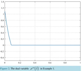
[image:7.595.171.454.495.702.2]

By numerical methods of two-point boundary value problems [18][19], we can obtain the optimal solution uˆ and the dual variable ρopt

( )

λˆ as follows (see Figure 1, Figure 2).

(8)

[image:8.595.173.459.83.333.2]

Figure 2. The dual variable ρopt

( )

λˆ in Example 1.

3. Box Constrained Optimal Control Problem

In this section, we consider U =

{

u t

( )

∈m − ≤1 u ti

( )

≤1,i=1, 2,,m

}

, t∈ t t0, f, and U is a unit box. Using the similar method in Section 2, the analytic solution to the box constrained optimal control problem

( )

 can be derived.

3.1. Global Optimization with Box Constraints

Similarly, consider the general box constrained problem

( )

{

}

minP u s t u. . ∈U U, = − ≤1 u_i≤1,i=1, 2,,m , (32) where P u

( )

is assumed to be twice continuously differentiable in m.

Denote

( )

{

2

}

0, 0, for every ,

m

P u Diag u U

ρ



ρ



ρ

= ∈ _∇ + _> ≥ ∈

 

where ρ=

(

ρ ρ₁, ₂,,ρ_m

)

T and Diag

( )

ρ

∈m m× is a diagonal matrix with ρ =i,i 1, 2,,m, being its di-agonal elements. It is obvious that if ρ ∈ˆ , then

ρ

∈ for any ρ ρ≥ ˆ. Parallel to what we did before, a differential flow uˆ

( )

ρ

is given as follow.

Assumed that ρ∗∈ and a nonzero vector u∗∈U such that

( )

0,

P u∗ Diag ρ∗ u∗

∇ + = (33) we focus on the flow uˆ

( )

ρ which is well defined near ρ∗

( )

* *1 1 1 2 2 2

ˆ ˆ ˆ ˆ

d d d d ,

ˆ , 1, 2, , ,

i i i im m m

i i

u H u H u H u

u u i m

ρ ρ ρ ρ ρ ρ ρ ρ

= + + +

 

= =





 (34)

where

(

_,_ˆ

( )

)

( )

2

(

_ˆ

( )

)

( )

1

ij _{m m}

H ρ u ρ H ρ P u ρ Diag ρ −

×  

 

=_ _ = − ∇_ + _ and uˆ

( )

ρ

=

(

uˆ₁

( ) ( )

ρ

,uˆ₂

ρ

,,uˆm

( )

ρ

)

T .

Moreover, near ρ∗, the differential flow uˆ

( )

ρ also satisfies

( )

(

ˆ

)

( ) ( )

ˆ 0.

P u ρ Diag ρ u ρ

(9)

canonical dual function is defined as follows

( )

(

( )

)

2

( )

1

ˆ ˆ 1 ,

2 m

d i

i i

P ρ P u ρ ρ u ρ

=

 

= +

∑

_ − _ (36) and the canonical dual problem associated with the problem (32) can be formulated as follows

( )

(

( )

)

2

( )

1

ˆ ˆ

: max 1 .

2

m

d d i

i i

P P ρ P u ρ ρ u ρ ρ

=

 ₌ ₊ _ ₋ _ _∈ 

 _ _ 



∑

 (37)

( )

ρ be a given flow defined by (33)-(34), and Pd

( )

ρ

be the corresponding canonical

dual function defined by (36). Near ρ∗, we have

( )

2

( )

2

( )

2

( )

T

1 2

1 1 1

ˆ 1 , ˆ 1 , , ˆ 1 ,

2 2 2

d

m

P ρ  u ρ  u ρ  u ρ 

∇ =_ _ − _ _ − _ _ − __

   (38)

( )

(

( )

)

(

( )

)

( )

1

(

( )

)

2 _ˆ 2 _ˆ _ˆ

. d

P ρ Diag u ρ  P u ρ Diag ρ − Diag u ρ

∇ = − _∇ + _ (39)

Proof. Since Pd

( )

ρ

is differentiable, near ρ∗,

( )

₍

_{( )}

₎

( )

_{( )}

( )

(

)

( )

(

( )

)

( )

(

)

( ) ( )

(

)

( )

T ₂ =1

T _T ₂

T ₂

ˆ

ˆ 1

ˆ ˆ 1 ˆ

2

ˆ ˆ 1

ˆ ˆ ˆ 1

2

ˆ 1

ˆ ˆ ˆ 1 .

2

d _m

j

i j j

j

i i i

i i i i i u P u

P u u u

u u

P u Diag u u

u

P u Diag u u

ρ

ρ ρ

ρ ρ ρ ρ

ρ ρ ρ

ρ ρ

ρ ρ ρ ρ

ρ ρ

ρ

ρ ρ ρ ρ

ρ ∂ ∂ ∂ _ _ = ∇ + _ − +_ ∂ ∂ ∂ ∂ ∂   = ∇ + + _ − _ ∂ ∂ ∂   = ∇ + + _ − _ ∂

∑

By (35), it follows that

( )

1 _ˆ2

( )

₁

2 d i i P u ρ ρ ρ ∂ _ _ = _ − _ ∂ .

Form (34), we have ˆi

( )

_ij

( ) ( )

ˆ_j j u H u ρ ρ ρ ρ ∂ =

∂ , then

( )

_{( ) ( )}

_{( ) ( ) ( )}

2

ˆ

ˆ ˆ ˆ .

d

i

i i ij j

i j j

P u

u u H u

ρ ρ

ρ ρ ρ ρ

ρ ρ ρ

∂ ∂

= =

∂ ∂ ∂

By the definition of H

(

ρ,uˆ

( )

ρ

)

, this concludes the proof of Lemma 5.

Lemma 5 shows that the canonical dual function Pd

( )

ρ

is concave on , so, the problem

( )

Pd can be solved by any commonly used nonlinear programming methods.

Theorem 4. (Perfect duality theorem) The canonical dual problem

( )

Pd is perfectly dual to the primal prob- lem (32) in the sense that if

ρ

∗∈ is a critical point of Pd

( )

ρ

, then the vector u∗=uˆ

( )

ρ∗ is a KKT point of (32) and P u

( )

∗ =Pd

( )

ρ∗ .

Proof. By the KKT theory, ρ∗ is a KKT point of

( )

Pd if and only if there exists one multiplier λ ∈m

such that

( )

* T * *

0, 0, 0, 0,

d

P ρ λ λ ρ λ ρ

∇ − = = ≤ ≥ (40)

( )

* 2

( )

* 2

( )

* 2

( )

* T

1 2

1 1 1

ˆ 1 , ˆ 1 , , ˆ 1 ,

2 2 2

d

m

P ρ  u ρ  u ρ  u ρ 

∇ =_ _ − _ _ − _ _ − __

  

where uˆ

( )

ρ is defined as (33)-(34). This shows that uˆ

( )

ρ∗ is a KKT point of the primal problem (32). By the complementarity conditions (40), we have

( )

(

( )

)

2

( )

(

( )

)

( )

1

ˆ ˆ 1 ˆ .

2

m

d i

i i

P ρ P u ρ ρ u ρ P u ρ P u

∗

∗ ∗ ∗ ∗ ∗

=

 

= +

∑

_ − =_ =

(10)

Theorem 5. (Triality theorem) Consider P u

( )

to be concave on the box U. If the flow uˆ

( )

ρ

defined by

(33)-(35) meets a boundary point of U at ρ ∈ˆ  such that uˆ_i2

( )

ρ

ˆ =1,i=1, 2,,m, then uˆ=uˆ

( )

ρ

ˆ is a global minimizer of the problem (32). Further one has

( )

(

( )

)

( )

ˆ

ˆ ˆ

ˆ

min d max d .

u U∈ P u =P u ρ =P ρ = ρ ρ≥ P ρ (41)

Proof. By Lemma 5 and the fact that uˆi2

( )

ρ

ˆ =1,

ρ

ˆ∈, it can verify that

( )

2

0

d

P

ρ

∇ ≤ and ∇Pd

( )

ρ

is monotonously decreasing as ρ ρ≥ ˆ. This means that uˆ

( )

ρ will stay in U and d

( )

d

( )

ˆ

P

ρ

≤P

ρ

as ρ ρ≥ ˆ. Using the definition of uˆ

( )

ρ as well as , we have

( )

(

)

2

( )

(

( )

)

( ) ( )

1

ˆ ˆ 1 ˆ ˆ 0,

2

m i

i i

P u ρ ρ u ρ P u ρ Diag ρ u ρ

=  _ _ ∇ + _ − _= ∇ + = 

∑

 

( )

(

)

( )

2 2 2

1

1 0, .

2

m i

i i

P u ρ u P u Diag ρ u U

=

 

∇ _ + − _= ∇ + > ∀ ∈



∑

 (42)

In the following deducing, we need to note the fact that since P u

( )

is twice continuously differentiable on

m

 , there exists a positive real vector δ ∈_m_{such that (42) holds in}

{

2

}

1

i i

u < +δ which contains U. So, we can show that uˆ

( )

ρ is the global minimizer of

( )

(

2

)

1 1 2 m i i i

P u ρ u

=

+

∑

− on U, and for any ρ ρ≥ ˆ

( )

(

)

( )

(

)

( )

(

)

( )

2 2 1 1 2 1

1 inf 1

2 2

ˆ ˆ 1 .

2 m m i i i i U i i m d i i i

P u P u u P u u

P u u P

ρ ρ

ρ

ρ ρ ρ

= = =   ≥ + − ≥  + −     _ _ = + _ − _=  

∑

(43)

Thus, we have

( )

(

( )

)

2

( )

(

( )

)

ˆ

1

ˆ

ˆ ˆ ˆ ˆ ˆ ˆ ˆ

max 1 .

2 m

d d i

i i

P u P P P u u P u

ρ ρ

ρ

ρ ρ ρ ρ ρ

≥ ₌  

≥ = = +

∑

_ − =_ (44)

By (43), (44) and the canonical duality theory, it leads to the conclusion we desired.

3.2. Analytic Solution to the Box Constrained Optimal Control Problem

Now, let

( )

1 T ˆT

( )

2

P u = u Ru+

λ

t Bu in (32). For

ρ

∈ =

{

ρ

∈m

ρ

i∈

[

0,+∞

)

,i=1, 2,,m

}

(since R is a positive definite matrix), we define

( )

1 _T

( )

0 ˆ

ˆ , a.e. , f ,

u

ρ

= −_R+Diag

ρ

_− B

λ

t t∈_t t _ (45) and the canonical dual function

( )

1 _T

( )

1 _T

( )

1 _T

ˆ ˆ _.

2 2

d

P

ρ

= −

λ

t B R_ +Diag

ρ

_− B

λ

t − e

ρ

(46) Set

( )

( ) ( )

(

2

( ) ( )

2 2

( )

)

T

1 2

ˆ ˆ ˆ ,ˆ , ,ˆ_m

y ρ =u ρ u ρ = u ρ u ρ u ρ (the notation “” denotes the Madamard product).

( )

ρ be a given flow defined by (45), and y

( )

ρ =uˆ

( ) ( )

ρ uˆ ρ . y_i

( )

ρ is monotonously decreasing with respect to ρ_i on

[

0,+∞

)

, i=1, 2,,m.

Proof. Notice that y_i

( )

ρ

=uˆ_i2

( )

ρ

and i

( )

2ˆi

( ) ( )

ˆi

i i

y u

u

ρ _ρ ρ

ρ ρ

∂ ∂

=

∂ ∂ . Let

(

( )

)

( )

1 ˆ

,

H

ρ

u

ρ

= −_R Diag+

ρ

_− and

( )

ii

H ρ be the ith diagonal element of H.

By properties of the positive definite matrix, it follows that the diagonal element H_ii

( )

ρ is a negative real number which means that i

( )

2 ii

( ) ( )

ˆi2 0

i y H u ρ ρ ρ ρ ∂ = ≤

∂ because of the fact that

( )

_{( ) ( )}

ˆ ˆ i ii i i u H u ρ ρ ρ ρ ∂ =

∂ . Thus,

(11)

In the rest part of this section, we suppose that R=Diag r

( )

is a diagonal matrix with ri>0,i=1, 2,, ,m being the diagonal elements. We have the following result.

Theorem 6. For the box constrained optimal control problem

( )

 , the analytic solution expressed by the

co-state is given as follows

( )

T T T T 1 2

T T T

1 2

ˆ

ˆ ˆ

ˆ , , , .

ˆ ˆ ˆ

max , max , max ,

m m m B B B u

r B r B r B

λ

λ λ

λ λ λ

 

 

= −  _ _ _ _ _ _  __ __ __ __ __ __

 

 (47)

Proof. Set

( )

(

( )

)

(

( )

)

(

( )

)

T

T T T T

1 2

ˆ ˆ _, ˆ _, _, ˆ

m

B

λ

t = B

λ

t B

λ

t  B

λ

t . It comes from Lemma 3.2 and (45) that

( )

(

( )

)

T_ˆ ˆ i i i i B t u r λ ρ ρ = − + ,

( )

(

)

(

)

2 T 2 ˆ i i i i B t y r λ ρ ρ =

+ and

( )

(

( )

)

(

)

2 T 3 ˆ 2 i i

i i i

B t y r λ ρ ρ ρ ∂ = − ∂ + ,

( )

0, i j y i j ρ ρ ∂ = ≠

∂ . This means that

( )

ˆ_i

u ρ and y_i

( )

ρ depend only on the element ρ_i, i.e. uˆ_i

( )

ρ =uˆ_i

( )

ρ_i and y_i

( )

ρ =y_i

( )

ρ_i .

Consider complementarity conditions ρ_i

(

y_i

( )

ρ − =1

)

0,i=1, 2,, .m If yi

( )

ρ >1 at the point ρ =i 0, by

Lemma 6, it is easy to verify that there must exist one point ρ >ˆi 0 such that

( )

(

)

(

)

2 T 2 ˆ 1 ˆ i i i B t r λ ρ =

+ . Otherwise, for any ρ ≥i 0, we always have yi

( )

ρ ≤1. Thus, we define the vector

opt m

ρ ∈ ,

( )

(

)

(

( )

)

( )

(

)

T T 0 T

ˆ _if ˆ _,

a.e. , ,

ˆ

0 if ,

i i i i opt i f i i

B t r B t r

t t t

B t r

λ λ

ρ

λ

 ₋ _>

 _ _

=_ ∈_ _

 ≤



(48)

which can be rewritten as

(

T

( )

)

0 ˆ

max 0, , a.e. ,

opt

i i f

i

B t r t t t

ρ = _ λ − _ _{∈ } _

  . It follows form (45) and (48) that a.e.

0, f

t∈ t t _,

( )

(

( )

)

( )

(

)

T T ˆ

ˆ , 1, 2, , .

ˆ max , opt i i i i B t

u i m

r B t

λ ρ λ = − =       

In what follows, parallel to the proof of Theorem 2, we shall show that ˆ

( )

opt

u ρ is the analytic solution for the problem

( )

 .

By statements as the above and Lemma 6, we have uˆ

( )

ρ ∈U for any ρ ρ_≥ opt_{, and the function family}

( )

{

fρ u

}

is given as follows

( )

(

2

)

T T

( )

(

2

)

1 1

1 _ˆ

1 1 ,

2 2 2

m m

i i

f_ρ u P u ρ u u Ru λ t Bu ρ u

= =

= +

∑

− = + +

∑

− (49)

where ρ is a parameter. Using (45) and (49), it is obvious that uˆ

( )

ρ is a global minimizer of the problem

( )

min f_ρ u on U by the fact that ∇fρ

(

uˆ

( )

ρ

)

=0 and ∇2fρ

( )

u > ∀ ∈0, u U. Further, we have

( )

inf

( )

(

ˆ

( )

opt

)

d

( )

opt . U

P u ≥ f_ρ u ≥ f_ρ u = f_ρ u ρ =P ρ (50) By Lemma 5 and (46), we have

( )

max

( )

(

ˆ

( )

)

. opt

d d opt opt

P u P P P u

ρ ρ≥ ρ ρ ρ

≥ = = (51)

Thus, _uˆ

( )

ρopt _{is a global minimizer of the problem (7). Consider}ρopt_{as a function with respect to the co-state}

ˆ

(12)

3.3. Applications

We will give an example to illustrate our results.

Example 2: For the box constrained optimal control problem

( )

 , we consider 2 7

2.5 3

A=  _

−

 ,

2 5

1.5 7

B=  − _

 ,

2.4 3

2 1

Q=  _

− −  ,

2 0 0 3

R=  _

 ,

( ) ( )

T

0 1,1

x = , t₀=0, and t_f =1, where Q≥0, R>0 sa-tisfying the assumption in (1).

[image:12.595.174.454.232.443.2]

Following idea of Lemma 1 and Theorem 2 as above, we need to solve a system on the state and co-state for deriving the optimal solution

Figure 3. The optimal feedback control ˆu in Example 2.

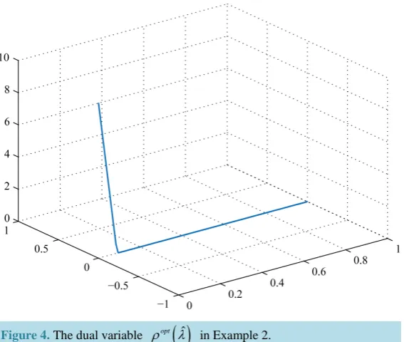
Figure 4. The dual variable ρopt

( )

λˆ

[image:12.595.173.457.475.715.2]

(13)

(

_ˆ

)

( ) ( )

T ˆ , , ,ˆ ˆ ˆ ˆ, ˆ 0 1,1 ,

x=H_λ t x u

λ

=Ax+Bu x = (52)

(

)

T

( )

ˆ _{, , ,}_{ˆ ˆ} ˆ ˆ _ˆ_, ˆ ₁ _0, x

H t x u A Qx

λ= − λ = − λ− λ = (53) and

( )

(

( )

)

( )

(

)

( )

(

)

( )

(

)

[ ]

T T

1 2

T T

1 2

ˆ ˆ

ˆ , ˆ , a.e. 0,1 .

ˆ ˆ

max 2, max 3,

B t B t

u t u t t

B t B t

λ λ

= − = − ∈

   

   

   

(54)

By solving Equations (52)-(54) in MATLAB, we can obtain the optimal optimal feedback control uˆ and the dual variable

ρ

opt

( )

λ

ˆ as follows (see Figure 3, Figure 4).

Acknowledgements

We thank the Editor and the referee for their comments. Research of D. Wu is supported by the National Science Foundation of China under grants No.11426091, 11471102.

References

[1] Casti, J. (1980) The Linear-Quadratic Control Problem: Some Recent Results and Outstanding Problems. SIAM Review,

22, 459-485. http://dx.doi.org/10.1137/1022089

[2] Robinson, C. (1995) Dynamical Systems. CRC Press, London.

[3] Anderson, B.D.O. and Moore, J.B. (1971) Linear Optimal Control. Prentice-Hall, New Jersey.

[4] Heinkenschloss, M. and Tröltzsch. F. (1999) Analysis of the Lagrange-SQP-Newton Method for the Control of a Phase Field Equation. Control and Cybernetics, 28, 177-211.

[5] Kunisch, K. and Sachs, E.W. (1992) Reduced SQP Methods for Parameter Identification Problems. SIAM Journal on Numerical Analysis, 29, 1793-1820. http://dx.doi.org/10.1137/0729100

[6] Tröltzsch, F. (1994) An SQP-Method for Optimal Control of a Nonlinear Heat Equation. Control and Cybernetics, 23, 268-288.

[7] Tian, T. and Dunn, J.C. (1994) On the Gradient Projection Method for Optimal Control Problems with Nonnegative L2

inputs. SIAM Journal on Control and Optimization, 32, 516-537.

[8] Kelley, C.T. and Sachs, E.W. (1995) Solution of Optimal Control Problems by a Pointwise Projected Newton Method.

SIAM Journal on Control and Optimization, 33, 1731-1757. http://dx.doi.org/10.1137/S0363012993249900

[9] Gao, D.Y., Ruan, N. and Latorre, V. (2014) Canonical Duality-Triality Theory: Bridge between Nonconvex Analysis/ Mechanics and Global Optimization in Complex Systems. Mathematics and Mechanics of Solids, 12, 716-735. [10] Gao, D.Y. and Ruan, N. (2015) Canonical Duality Theory for Solving Nonconvex/Discrete Constrained Global

Opti-mization Problems. Mathematics and Mechanics of Solids. http://dx.doi.org/10.1177/1081286515591087

[11] Latorre, V. and Sagratella, S. (2014) A Canonical Duality Approach for the Solution of Affine Quasi-Variational In-equalities. Journal of Global Optimization, 1, 1-17.

[12] Gao, D.Y. and Ruan, N. (2015) Application of Canonical Duality Theory to Fixed Point Problem. Springer Proceed-ings in Mathematics & Statistics, 95, 157-163. http://dx.doi.org/10.1007/978-3-319-08377-3_17

[13] Zhu, J., Tao, S. and Gao, D.Y. (2009) A Study on Concave Optimization via Canonical Dual Function. Journal of Computational and Applied Mathematics, 224, 459-464. http://dx.doi.org/10.1016/j.cam.2008.05.011

[14] Zhu, J. and Yan, W. (2009) Solution to Constrained Nonlinear Programming by Canonical Dual Method. Lecture Notes on Decision Sciences, 12, 217-222.

[15] Zhu, J., Wu, D. and Gao, D.Y. (2012) Applying the Canonical Dual Theory in Optimal Control Problems. Journal of Global Optimization, 29, 377-399. http://dx.doi.org/10.1007/s10898-009-9474-3

[16] Adjiman, C.S., Androulakis, I.P. and Floudas, C.A. (1998) A Global Optimization Method, αBB, for General Twice- Differentiable Constrained NLPs—II. Implementation and Computational Results. Computers & Chemical Engineer-ing, 22, 1159-1179. http://dx.doi.org/10.1016/S0098-1354(98)00218-X

[17] Adjiman, C.S., Androulakis, I.P. and Floudas, C.A. (1998) A Global Optimization Method, αBB, for General Twice- Differentiable Constrained NLPs—I. Theoretical Advances. Computers & Chemical Engineering, 22, 1137-1158.

(14)

[18] Keller, H.B. (1976) Numerical Solution of Two Point Boundary Value Problems. SIAM, Philadelphia.

http://dx.doi.org/10.1137/1.9781611970449

[19] Ascher, U.M., Mattheij, R.M.M. and Russell, R.D. (1995) Numerical Solution of Boundary Value Problems for Ordi-nary Differential Equations (Classics in Applied Mathematics). SIAM, Philadelphia.