ARFIMAX and ARFIMAX TARCH Realized Volatility Modeling

Munich Personal RePEc Archive

ARFIMAX and ARFIMAX-TARCH

Realized Volatility Modeling

Degiannakis, Stavros

Department of Statistics, Athens University of Economics and

Business

2008

Online at

https://mpra.ub.uni-muenchen.de/80465/

A R F I M A X a n d A R F I M A X - T A R C H R e a l i z e d V o l a t i l i t y M o d e l i n g

Stavros Degiannakis

Department of Statistics, Athens University of Economics and Business

A b s t r a c t

ARFIMAX models are applied in estimating the intra-day realized volatility of the

CAC40 and DAX30 indices. Volatility clustering and asymmetry characterize the logarithmic

realized volatility of both indices. ARFIMAX model with time-varying conditional

heteroscedasticity is the best performing specification and, at least in the case of DAX30,

provides statistically superior next trading day’s realized volatility forecasts.

Keywords: ARFIMAX, Realized Volatility, TARCH, Volatility Forecasting.

1 . I n t r o d u c t i o n

Andersen and Bollerslev (1998) first stated that the volatility estimates based on intra-day

returns are more accurate than those based one daily data and introduced the realized volatility. The concept of the realized volatility is based on the integrated volatility. The integrated

volatility,  IV t

2

 , aggregated over the time interval



t1,t



:

 

_{ }

dx x t t IV t 2 1 2  

_



 , (1)

is a latent variable which is not observable. Integrated volatility’s volatility named integrated

quarticity is  



 





t

t IQ

t x dx

1 4

2 ₂

 . The integrated volatility is asymptotically normally distributed:

 

_{ }

 

 

0,1 2 1 4 1 2 2 N dx x dx x m d t t t t IV t        





    

.1 ₍₂₎

The volatility at a lower frequency is computed using data available at a higher frequency. Thus,

the integrated volatility over the time interval



t1,t



can be consistently estimated by the

trading day’s t realized volatility,  







_{ }





_{ }





     1 1 2 , , 1 2 log log m j t m j t m j RV

t P P

 , which is defined as the

sum of squared log-returns observed over m intra-day time intervals, for

 

P_{ }m,t m_j1 denoting the

asset prices over m intra-day time intervals of day t. The realized volatility converges in

probability to the integrated volatility as m, or

 







 







 IV

t m j t m j t m j m P P p 2 1 1 2 , , 1 log log

lim _

     



    . 2

Fractionally integrated autoregressive moving average with exogenous variables

(ARFIMAX) models, introduced by Granger (1980), were proposed to model the long memory

property of the realized volatility. Ebens (1999) proposed the application of ARFIMAX models

in realized volatility modelling and they, subsequently, applied by Bollerslev and Wright (2001),

Giot and Laurent (2004), Koopman et al. (2005) and Angelidis and Degiannakis (2009) among

others. As concerns the point forecasts of volatility, the findings provide evidence in favour of

1 _{For details about}  IV t 2

 and  IQ t

2

 see Barndorff-Nielsen and Shephard (2005) and references therein.

realized volatility ARFIMAX models rather than autoregressive conditional heteroskedasticity

(ARCH) framework of modeling daily log-returns. Corsi et al. (2005) noted that the volatility of

S&P500 index futures volatility also exhibits time-variation and proposed the estimation of an

ARFIMAX model that accounts for conditional heteroskedasticity.

In the present study, an ARFIMAX model is extended to account for volatility clustering

as well as for the asymmetric relation between realized volatility and volatility of realized

volatility. The unobservable term of an ARFIMAX specification is modelled as an asymmetric

ARCH process. The new model framework, named ARFIMAX-TARCH model, is applied for

CAC40 and DAX30 stock indices. In-sample as well as out-of-sample analysis provide

statistically significant evidence in favour of the new model specification. Thus, in risk

management applications, the volatility’s conditional volatility should be taken into

consideration.

The manuscript is divided in six sections. In section 2, descriptive information of the

CAC40 and DAX30 realized volatility measures is provided. Section 3 lays out the ARFIMAX

and ARFIMAX-TARCH specifications. The in-sample and out-of-sample model evaluation is

investigated in sections 4 and 5, respectively, and section 6 concludes.

2 . C A C 4 0 a n d D A X 3 0 R e a l i z e d V o l a t i l i t y P r o p e r t i e s

Tick by tick linearly interpolated prices of the CAC40 and DAX30 indices were obtained

from Olsen and Associates for the period of July 1995 to December 2003. The sampling

frequency should be as high as the market microstructure features do not induce bias to volatility

estimator. In order to avoid market microstructure frictions without lessening the accuracy of the

continuous record asymptotics, in most of the studies, such as Andersen and Bollerslev (1998),

Andersen et al. (1999, 2001b) and Kayahan et al. (2002), a sampling frequency of five minutes is

used.

The realized intraday volatility at day t is computed as in Martens (2002) and Koopman et al. (2005):

 

 







 











 

 

 1

1

2 , ,

1 2

2 2

2 _{log log}

ˆ ˆ

ˆ m

j

t m j t

m j oc

co oc RV

t  P P

 

 , (3)

where

 

P_{ }m,t m_j1 are the five-minute linearly interpolated prices at trading day t with

103



m



m134



observations per day for the CAC40 (DAX30) index,

 

 



 











 _

 T

t

t m t

oc T P P

1

2 , 1 ,

1 1

2

log log

ˆ

 







 









 

 _

 T

t

t t

m

co T P P

1

2 1 , 1 ,

1 1

2

log log

ˆ

 is the close to open sample variance. The factor



2 2



2

co oc oc  

 

accounts for changes in the asset prices during the hours that the stock market is

closed without inserting the noisy effect of daily returns.

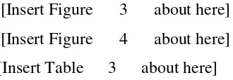
[Insert Table 1 about here]

Table 1 lists descriptive information of the logarithmic realized volatility,



 RV



t

2

log .

Lilliefors’ (1967) and Anderson and Darling’s (1954) statistics reject the null hypothesis that the

logarithmic realized variance is normally distributed. Literature provides empirical evidence that

the distribution of the daily returns, yt log



Pt Pt1



, standardized by the square root of the

realized volatility,



 RV



T_t t t

y  _1, is very close to the normal one, but, it is statistically

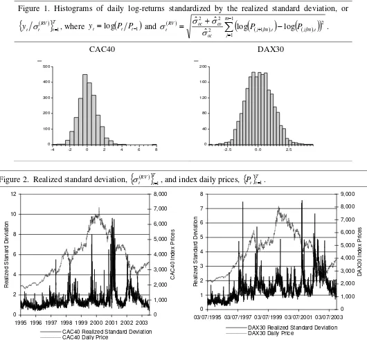
distinguishable from the normal distribution3. The histograms of



 



Tt RV t t

y  _1 are plotted in

Figure 1. According to Lilliefors and Aderson-Darling normality tests in Table 3,



 RV



T_t t t

y  _1 is

normally distributed, in the case of DAX30, at 1% level of significance. In the case of CAC40,

the null hypothesis, that the empirical distribution of



 RV



T_t t t

y  _1 is the normal one, is rejected at

any reasonable level of significance.

Figure 2 presents the square root of realized volatility. On the right-hand axis, the daily

index prices are plotted to present the asymmetric relationship between index log-returns and

changes in realized volatility.

[Insert Figure 1 about here]

[Insert Figure 2 about here]

3 . A R F I M A X a n d A R F I M A X - T A R C H I n t r a - D a y V o l a t i l i t y M o d e l s

An ARFIMAX



k,d,l



model for the realized volatility,  RV t

2

 , can be presented as:

 











 





_

_{ }

_

t t

RV t d

L x

L L

c       

 1 log 1

1 2 ,

 

2

, 0

~ _

_t N ,

(4)

where

 



  k i i iL c L c 1 ,

 



  l i i iL L 1 

 , L is the backward-shift operator,





_

_



_{  }



_

_

                j k j j j j d k d k L d j L d j L 0 0 0 1 1

1 , 



. is the Gamma function, xt is a vector of

explanatory variables and  is a vector of unknown parameters.

As, we want to investigate whether the volatility of realized volatility exhibits

time-variation, the ARFIMAX model is extended to account for conditional heteroskedasticity4. An ARFIMAX model with time varying conditional variance for the realized volatility,  RV

t 2

 , can

be presented as:

 











 







 







 

0,1, ~ | 1 log 1 1 1 2 2 N z I g z L x L L c t t t t t t t t RV t d                  (5)

where It1 is the information set available in time t1, 2 t

 is a time-varying, positive and

measurable function of It1,  is a vector of unknown parameters and g



. is a functional form of

1  t

I . In our case, an asymmetric conditional variance specification is considered to account for

asymmetric relationship between realized volatility and its volatility. Therefore an

ARFIMAX



k,d,l



-TARCH

 

p,q model for the realized volatility is proposed:

 











 





_

_{ }

_

t t RV t d L x L L

c       

 1 log 1

1 2 ,

t t t  z   ,









_





            p i i t i q i i t i t i q i i t i

t a a I b

1 2 1 2 1 2 0 2

0 

  

 ,

(6)

where z_t ~N

 

0,1 . I



. denotes the indicator function, i.e. I



ti 0



1 if ti 0, and



ti 0



0

I  , otherwise. The Threshold-ARCH

 

p,q , or TARCH

 

p,q , specification,

introduced by Glosten et al. (1993), allows positive,



ti 0



, and negative,



ti 0



,

innovations to have differential effects on the volatility of the realized volatility.

4 . I n - s a m p l e E v a l u a t i o n

The ARFIMAX



k,d,l



model is considered in the form:

4 _{Baillie et al. (1996) firstly proposed an ARFIMAX–ARCH model to analyze monthly consumer price index inflation. Hauser}

 











 



_

_



_

_{ }

_



0,



, ~ , 1 0 log 1 1 2 1 1 2 1 1 0 2       N L y y I w y w w L L c t t t t t RV t

d _{     }



 _{  }

(7)

where I



yt 0



1 when yt 0 and I



yt 0



0 otherwise. Parameter w2 models the

asymmetric relationship between realized volatility and previous trading day’s log-return5. Since,

 

2

, 0

~ _

_t N , the exp

 

t is log-normally distributed, therefore the unbiased in-sample realized

volatility is estimated as:

 



2  2



2 5 . 0 ˆ log exp ˆ *   

  RV 

t RV

t . (8)

In order to determine the optimal lag order, model (7) is estimated for k0,1,2 and

2 , 1 , 0 

l . The optimal lag order is chosen due to the minimization of Schwarz’s (1978) Bayesian

criterion (SBC). The SBC, for model i, is computed as:

 



_{ }

 



_{ }

log

ˆ

;

2T 1L y T 1 T

SBCi   _{T t}  T   , (9)

where  



c1,...,ck,d,w0,w1,w2,1,...,l



, LT



. is the maximized value of the log-likelihood

function, ˆ T

is the maximum likelihood estimator of  based on a sample of size T and 

denotes the dimension of  . The optimal lag orders are ARFIMAX



2,d,2



and

ARFIMAX



0,d,1



for CAC40 and DAX30, respectively. The models are estimated in Doornik

and Ooms’ (2006) ARFIMA 1.04 package of Ox Metrics.

The ARFIMAX



k,d,l



-TARCH

 

p,q model is also considered in the form:

 











 



_

_



_

_{ }

_

t t t t RV t d L y y I w y w w L L

c         

 1 log _{ } 0 _ 1

1 0 1 1 2 1 1

2

,

t t t  z   ,









_





            p i i t i q i i t i t i q i i t i

t a a I b

1 2 1 2 1 2 0 2

0 

  

 ,

 

0,1

~N

z_t .

(10)

Model (10) is estimated for k0,1,2, l0,1,2, p0,1,2 and q1,2. The SBC is computed

according to equation (9) for  



c1,...,ck,d,w0,w1,w2,1,...,l,a0,a1,...,aq,1,...,q,b1,...,bp



.

The ARFIMAX



1,d,1



-TARCH

 

1 model achieves the minimum value of the ,1 SBC criterion for

both indices. The unbiased in-sample realized volatility is also estimated according to (8). The

models are estimated in Laurent and Peters’ (2006) G@RCH 4.04 package for Ox Metrics.

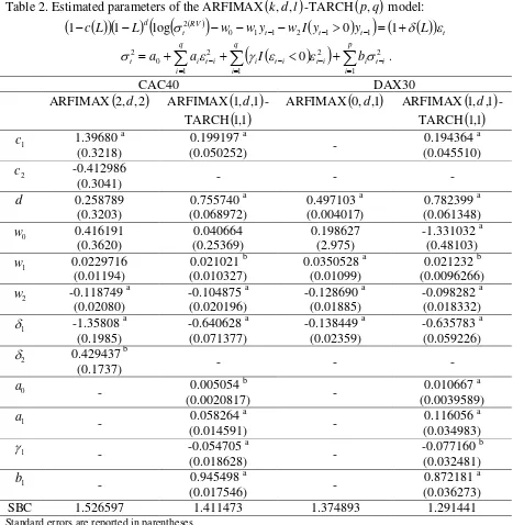
The estimated parameters of the models that minimize the SBC criterion are reported in

Table 2. Τhe values of the parameters inform us that i) the asymmetric relation between past

return and realized volatility is statistically significant in all cases (coefficient w₂), ii) the

fractional integration parameter is statistically insignificant only for Paris stock market in the

ARFIMAX



2,d,2



model (coefficient d), iii) all the conditional variance parameters are

statistically significant (coefficients a1 and b1), and iv) the asymmetric relationship between

realized volatility and its volatility is also statistically significant (coefficient ₁). The

significance of the conditional variance parameters justifies the modeling of realized volatility’s

conditional variance6.

[Insert Table 2 about here]

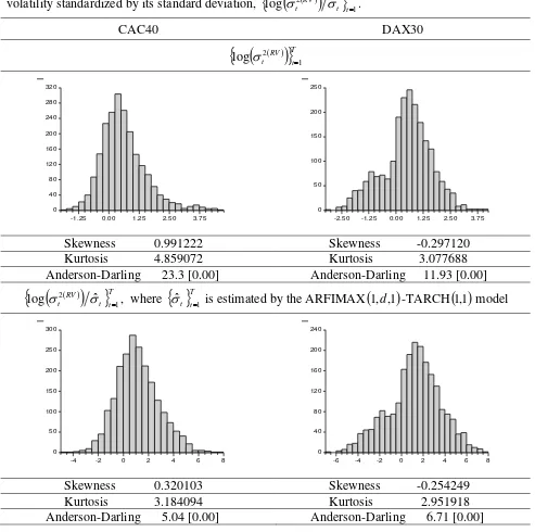
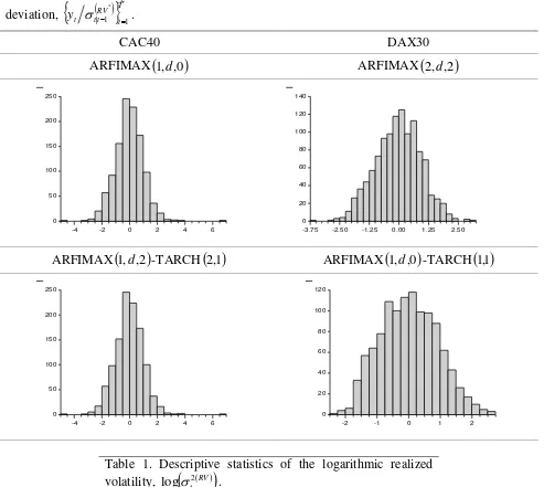
Figure 3 plots the histograms of logarithmic realized volatility,





 RV





T_t

t 1

2

log _ and

logarithmic realized volatility standardized by its standard deviation estimated by the

ARFIMAX



1,d,1



-TARCH

 

1 model, ,1





 



t



T_t RV

t 1

2 ˆ

log  _ . The





 



t



T_t

RV

t 1

2 ˆ

log  _ is much

closer to the normal distribution than the





 





Tt RV

t 1

2

log _ is, but it is statistically distinguishable

from it.

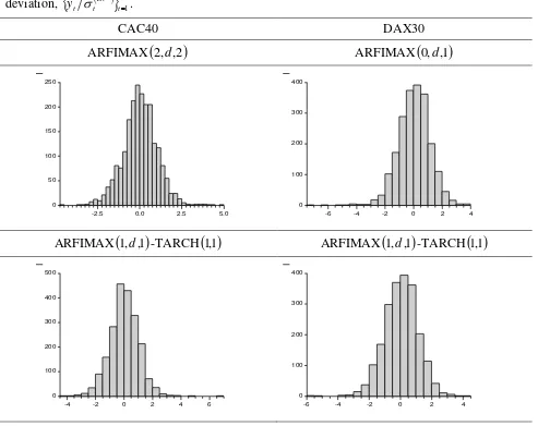
Figure 4 depicts the density graph of daily returns standardized by the in-sample

estimated realized standard deviation,



 



Tt RV t t

y ˆ * _1, whereas normality tests are listed in Table 3.

Based on Lilliefors statistic, the hypothesis that



 



Tt RV t t

y ˆ * _1 is normally distributed can not be rejected only in the case of DAX30 at 1% level of significance. Anderson-Darling statistic rejects

the normality in any case.

[Insert Figure 3 about here]

[Insert Figure 4 about here]

[Insert Table 3 about here]

The average squared distance between realized volatility and its in-sample estimation is

measured to evaluate the accuracy of the models in estimating the realized volatility:

   









 _

 T

t

RV t RV t

T MSE

1

2 2 2

1  ˆ *

. (11)

[image:8.595.204.369.563.620.2]

Hansen and Lunde (2006) have stated that the MSE loss function ensures the equivalence of the

ranking of volatility models that is induced by the true volatility and its proxy. The values of the

MSE loss functions are reported in Table 4. For both indices, the ARFIMAX



1,d,1



-TARCH

 

1 ,1

model has the lowest value.

Hansen’s (2005) superior predictive ability (SPA) hypothesis testing is used to investigate

whether the model with the lowest MSE value provides statistically superior realized volatility

estimates. Let i be the model with the lowest MSE value,  i* t

MSE is the value of the MSE

function at time t of a competing model _i*_{, for i}* _1,...,M

and  ,    i*

t i

t i

i

t MSE MSE

X    . The

null hypothesis that



 ,1, . . . , i,M



0

t i

t X

X

E is tested with the statistic







 _



i i M

i SPA

X M Var

X M T

,..., 1

max , where



 



 

  T

t i i t

i T X

X

1 , 1

.7

According to Table 4, the ARFIMAX-TARCH specification is superior to the ARFIMAX

one. The null hypothesis, that the ARFIMAX



1,d,1



-TARCH

 

1 model is not outperformed by ,1

its competing model, is not rejected.

[Insert Table 4 about here]

5 . O u t - o f - s a m p l e E v a l u a t i o n

In the present section, the ability of the ARFIMAX



k,d,l



and ARFIMAX



k,d,l



-TARCH

 

p,q models to predict next trading day’s volatility is investigated. In total, for

2 , 1 , 0



k , l 0,1,2, p0,1,2 and q1,2 lag orders, 56 model specifications are considered.

Based on a rolling sample of T1000 trading days, each model’s parameter vector  is

re-estimated every trading day and T~ one-day-ahead volatility forecasts are computed8, for

T T

T~  . The one-day-ahead conditional standard deviation forecasts are computed as:

 





 RV



 t



t

t RV

t t

2 2

| 1 |

1 explog 0.5

*



 

 _  _  . (12)

The distance between realized volatility and next day’s predicted volatility is measured by

the predicted mean squared error loss function:

7 _{The estimation of}







i

X M

Var and the p-value of the SPA

T are obtained by using the bootstrap method of Politis and Romano (1994). Hansen (2005) provided a program for the computation of the SPA criterion, which is written in Ox Metrics package.

   







  

 _

 T

t

RV t t RV t

T PMSE

~

1

2 2

| 1 2

1

1 *

~ _{ }

, (13)

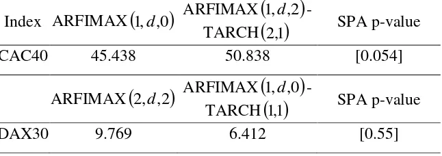
and the SPA hypothesis test is applied. In the ARFIMAX



k,d,l



specification, the PMSE is

minimized for k 1 and l0 in the CAC40 case, and for kl2 in the case of DAX30. In the ARFIMAX



k,d,l



-TARCH

 

p,q framework, the PMSE is minimized for k 1, l 2, p2,

1



q in the CAC40 case, and for k pq1, l 0 in the case of DAX30. Table 5 presents the p-values of the SPA test for the null hypothesis that the ARFIMAX-TARCH model is not

outperformed by the ARFIMAX one. In the case of the DAX30 the ARFIMAX



1,d,0



-TARCH

 

1 model is superior to the ARFIMAX,1



2,d,2



one. As concerns the CAC40 index, the

ARFIMAX



1,d,2



-TARCH

 

2,1 model does not achieve the lowest value in the PMSE loss

function, but it is not statistically inferior to its competitor, the ARFIMAX



1,d,0



model.

[Insert Table 5 about here]

Figure 5 presents the returns scaled by the one-day-ahead realized standard deviation

forecasts,



 RV



T_t t t t y

~ 1 1 |

*

 

 . According to Table 3, the null hypothesis, that the daily returns

standardized by the one-day-ahead realized standard deviation forecasts are normally distributed,

in not rejected only for the ARFIMAX



2,d,2



model in the DAX30 case. Giot and Laurent

(2004) noticed that for the CAC409 and SP500 indices, the



 RV



T_t t t

y  _1 are normally distributed,

but the



 RV



T_t t t t

y

1 1 |

*

 

 are not normally distributed. In the present dataset both series



 RV



T_t t t

y  _1

and



 RV



T_t t t t

y

1 1 |

*

 

 are not normally distributed but they have an almost normal distribution as in

Andersen et al. (2001a).

[Insert Figure 5 about here]

6 . C o n c l u s i o n

ARFIMAX and ARFIMAX-TARCH models were applied in estimating and forecasting

the intra-day realized volatility of the CAC40 and DAX30 indices for the period of July 1995 to

December 2003. ARFIMAX-TARCH model takes into consideration the dynamics of realized

volatility’s volatility. The integrated volatility,  IV t

2

 , is estimated by the realized volatility,

 RV t

2

 , in equation (3), whereas the conditional variance of the logarithmic realized volatility,

2

ˆt

 , in equatrion (10), can be regarded as an estimation of integrated quarticity,  IQ t

2

 . The

significance of the parameters of the TARCH specification provides evidence in favor of

modeling the asymmetric relationship between realized volatility and its volatility.

The in-sample evaluation indicates that the ARFIMAX-TARCH specification clearly

outperforms the ARFIMAX one. In the out-of-sample evaluation, the ARFIMAX-TARCH model

is superior to the ARFIMAX one for the DAX30. In the case of the CAC40 index, the

ARFIMAX-TARCH model is not statistically inferior to its competitor.

To sum up, from econometric point of view, the daily returns standardized by i) the

realized standard deviation, ii) the in-sample estimated realized standard deviation, and iii) the

one-day-ahead realized standard deviation forecasts are almost normally distributed but they are

statistically distinguishable from the normal distribution. The logarithmic realized volatility

standardized by its standard deviation is much closer to the normal distribution than the

logarithmic realized volatility but also statistically distinguishable from it.

From economic point of view, in order to obtain more accurate stock index volatility

estimations, it is necessary to treat ARFIMAX models for realized volatility, and ARCH

modeling for volatility of realized volatility, simultaneously. Thus, when the volatility estimation

is required in financial applications, such as risk management, option pricing and portfolio

analysis, the time varying conditional heteroscedasticity of volatility should be taken into

consideration.

R e f e r e n c e s

1. Andersen, T. and Bollerslev, T. (1998). Answering the Skeptics: Yes, Standard Volatility Models Do Provide Accurate Forecasts. International Economic Review, 39, pp. 885-905.

2. Andersen, T., Bollerslev, T. and Lange, S. (1999). Forecasting Financial Market Volatility: Sample Frequency vis-à-vis Forecast Horizon. Journal of Empirical Finance, 6, pp. 457-477.

3. Andersen, T., Bollerslev, T., Diebold, F.X. and Ebens, H. (2001a). The Distribution of Realized Stock Return Volatility. Journal of Financial Economics, 61, pp. 43-76.

4. Andersen, T., Bollerslev, T., Diebold, F.X. and Labys, P. (2001b). The Distribution of Exchange Rate Volatility. Journal of the American Statistical Association, 96, pp. 42-55.

6. Angelidis, T. and Degiannakis, S. (2009). Volatility Forecasting: Intra-day vs. Inter-day Models. Journal of International Financial Markets, Institutions and Money, forthcoming.

7. Baillie, R.T., Chung, C.F., and Tieslau, M.A. (1996). Analysing Inflation by the

Fractionally Integrated ARFIMA-GARCH Model. Journal of Applied Econometrics, 11, pp. 23–

40.

8. Barndorff-Nielsen, O.E. and Shephard, N. (2005). How Accurate is the Asymptotic Approximation to the Distribution of Realised Volatility? in D. Andrews, J. Powell, P. Ruud, and

J. Stock (Eds.) Identification and Inference for Econometric Models, Cambridge: Cambridge University Press.

9. Bollerslev, T. and Wright, J.H. (2001). Volatility Forecasting, High-Frequency Data and Frequency Domain Inference. Review of Economics and Statistics, 83, pp. 596-602.

10. Corsi, F., Kretschmer, U., Mittnik, S. and Pigorsch, C. (2005). The Volatility of Realised Volatility. Center for Financial Studies, Working Paper, 33.

11. Doornik, J.A. and Ooms, M. (2006). A Package for Estimating, Forecasting and Simulating Arfima Models: Arfima Package 1.04 for Ox. Nuffield College, Oxford, Working

Paper.

12. Ebens, H. (1999). Realized Stock Volatility. Johns Hopkins University, Department of Economics, Working Paper, 420.

13. Giot, P. and Laurent, S. (2004). Modelling Daily Value-at-Risk Using Realized Volatility and ARCH Type Models. Journal of Empirical Finance, 11, pp. 379 – 398.

14. Glosten, L., Jagannathan, R. and Runkle, D. (1993). On the Relation Between the Expected Value and the Volatility of the Nominal Excess Return on Stocks. Journal of Finance, 48, pp. 1779–1801.

15. Granger, C.W.J. (1980). Long Memory Relationships and the Aggregation of Dynamic Models. Journal of Econometrics, 14, pp. 227-238.

16. Hansen, P.R. (2005). A Test for Superior Predictive Ability. Journal of Business and Economic Statistics, 23, pp. 365-380.

17. Hansen, P.R. and Lunde, A. (2006). Consistent Ranking of Volatility Models. Journal of Econometrics, 131, pp. 97-121.

18. Hauser, M.A. and Kunst, R.M. (1998). Fractionally Integrated Models With ARCH Errors: With an Application to the Swiss 1-Month Euromarket Interest Rate. Review of

Quantitative Finance and Accounting, 10, pp. 95-113.

20. Kayahan, B., Saltoglu, T. and Stengos, T. (2002). Intra-Day Features of Realized Volatility: Evidence from an Emerging Market. International Journal of Business and

Economics, 1(1), pp. 17-24.

21. Koopman, S.J., Jungbacker, B., and Hol, E. (2005). Forecasting Daily Variability of the S&P100 Stock Index Using Historical, Realised and Implied Volatility Measurements.

Journal of Empirical Finance, 12, pp. 445–475.

22. Laurent S. and Peters, J.-P. (2006). G@RCH 4.2, Estimating and Forecasting ARCH Models, London: Timberlake Consultants Press.

23. Lilliefors, H.W. (1967). On the Kolmogorov-Smirnov Test for Normality with Mean and Variance Unknown. Journal of the American Statistical Association, 62, pp. 399-402.

24. Martens, M. (2002). Measuring and forecasting S&P500 index-futures volatility using high-frequency data. Journal of Futures Markets, 22, pp. 497–518.

25. Politis, D.N. and Romano, J.P. (1994). The Stationary Bootstrap. Journal of the American Statistical Association, 89, pp. 1303-1313.

Figures & Tables

Figure 1. Histograms of daily log-returns standardized by the realized standard deviation, or

 





T

t RV t t

y  _1, where yt log



Pt Pt1



and

   







 









      1 1 2 , , 1 2 2 2 log log ˆ ˆ ˆ m j t m j t m j oc co oc RV

t _ P P

 

 .

CAC40 DAX30

0 100 200 300 400 500

-4 -2 0 2 4 6 8

0 40 80 120 160 200

-2.5 0.0 2.5

Figure 2. Realized standard deviation,

 

 RV T_t t 1

 , and index daily prices,

 

Pt T_t1.

0 2 4 6 8 10 12

1995 1996 1997 1998 1999 2000 2001 2002 2003

R e a liz e d S ta n a rd D e v iat ion 0 1,000 2,000 3,000 4,000 5,000 6,000 7,000 8,000 C A C 4 0 I n d e x P ric e s

CAC40 Realized Standard Deviation CAC40 Daily Price

0 1 2 3 4 5 6 7 8

03/07/1995 03/07/1997 03/07/1999 03/07/2001 03/07/2003

R e a liz e d S ta n d a rd D e v iat ion 0 1,000 2,000 3,000 4,000 5,000 6,000 7,000 8,000 9,000 D A X 3 0 I n d e x P ric e s

[image:14.595.33.563.112.603.2]

[image:15.595.53.546.120.610.2]

Figure 3. Histogram of logarithmic realized volatility,





 RV





T_t

t 1

2

log _ , and of logarithmic realized

volatility standardized by its standard deviation,





 



t



T_t RV

t 1

2 ˆ

log  _ .

CAC40 DAX30

 









T

t RV

t 1

2

log _

0 40 80 120 160 200 240 280 320

-1.25 0.00 1.25 2.50 3.75

0 50 100 150 200 250

-2.50 -1.25 0.00 1.25 2.50 3.75

Skewness 0.991222 Skewness -0.297120

Kurtosis 4.859072 Kurtosis 3.077688

Anderson-Darling 23.3 [0.00] Anderson-Darling 11.93 [0.00]

 









T

t t RV

t 1

2 ˆ

log  _ , where

 

ˆt T_t1 is estimated by the ARFIMAX



1,d,1



-TARCH

 

1 model ,1

0 50 100 150 200 250 300

-4 -2 0 2 4 6 8

0 40 80 120 160 200 240

-6 -4 -2 0 2 4 6 8

Skewness 0.320103 Skewness -0.254249

Kurtosis 3.184094 Kurtosis 2.951918

[image:16.595.54.547.113.504.2]

Figure 4. Histogram of daily log-returns standardized by the in-sample estimated realized standard

deviation,



 



Tt RV t t

y ˆ * _1.

CAC40 DAX30

ARFIMAX



2,d,2



ARFIMAX



0,d,1



0 50 100 150 200 250

-2.5 0.0 2.5 5.0

0 100 200 300 400

-6 -4 -2 0 2 4

ARFIMAX



1,d,1



-TARCH

 

1 ,1 ARFIMAX



1,d,1



-TARCH

 

1 ,1

0 100 200 300 400 500

-4 -2 0 2 4 6

0 100 200 300 400

Figure 5. Histogram of daily log-returns standardized by the one-day-ahead realized standard

deviation,



 RV



T_t t t t y

~ 1 1 |

*

 

 .

CAC40 DAX30

ARFIMAX



1,d,0



ARFIMAX



2,d,2



0 50 100 150 200 250

-4 -2 0 2 4 6

0 20 40 60 80 100 120 140

-3.75 -2.50 -1.25 0.00 1.25 2.50

ARFIMAX



1,d,2



-TARCH

 

2,1 ARFIMAX



1,d,0



-TARCH

 

1 ,1

0 50 100 150 200 250

-4 -2 0 2 4 6

0 20 40 60 80 100 120

-2 -1 0 1 2

Table 1. Descriptive statistics of the logarithmic realized volatility,



 RV



t 2

log .

CAC40 DAX30

Mean 0.602 0.498

Median 0.479 0.567

Maximum 4.523 4.046

Minimum -1.751 -3.171

Std. Dev. 0.923 1.117

Skewness 0.9912 -0.2971

Kurtosis 4.8590 3.0776

Lilliefors 0.077 [0.00] 0.067 [0.00]

Anderson-Darling 23.3 [0.00] 11.93 [0.00]

[image:17.595.54.547.118.559.2] [image:17.595.147.453.565.758.2]

[image:18.595.65.532.88.566.2]

Table 2. Estimated parameters of the ARFIMAX



k,d,l



-TARCH

 

p,q model:

 











 



_

_



_

_{ }

_

t t t t RV t d L y y I w y w w L L

c         

 1 log _{ } 0 _ 1

1 0 1 1 2 1 1

2









_





            p i i t i q i i t i t i q i i t i

t a a I b

1 2 1 2 1 2 0 2

0 

  

 .

CAC40 DAX30

ARFIMAX



2,d,2



ARFIMAX



1,d,1



-TARCH

 

1 ,1

ARFIMAX



0,d,1



ARFIMAX



1,d,1



-TARCH

 

1 ,1

1

c 1.39680 a

(0.3218)

0.199197 a

(0.050252) -

0.194364 a (0.045510)

2

c -0.412986

(0.3041) - - -

d 0.258789

(0.3203)

0.755740 a (0.068972)

0.497103 a (0.004017)

0.782399 a (0.061348) 0 w 0.416191 (0.3620) 0.040664 (0.25369) 0.198627 (2.975)

-1.331032 a (0.48103)

1

w 0.0229716

(0.01194)

0.021021 b (0.010327)

0.0350528 a (0.01099)

0.021232 b (0.0096266)

2

w -0.118749 a

(0.02080)

-0.104875 a (0.020196)

-0.128690 a (0.01885)

-0.098282 a (0.018332)

1

 -1.35808 a

(0.1985)

-0.640628 a (0.071377)

-0.138449 a (0.02359)

-0.635783 a (0.059226)

2

 0.429437 b

(0.1737) - - -

0

a _- 0.005054 b

(0.0020817) -

0.010667 a (0.0039589)

1

a _- 0.058264 a

(0.014591) -

0.116056 a (0.034983)

1 

- -0.054705

a

(0.018628) -

-0.077160 b (0.032481)

1 b

- 0.945498

a

(0.017546) -

0.872181 a (0.036273)

SBC 1.526597 1.411473 1.374893 1.291441

Standard errors are reported in parentheses.

Table 3. Lilliefors and Anderson-Darling statistics for the hypothesis that the daily returns

standardized by i) the realized standard deviation,



 RV



T_t t t

y  _1, ii) the in-sample estimated

realized standard deviation,



 



Tt RV t t

y ˆ * _1, and ii) the one-day-ahead realized standard deviation

forecast,



 RV



T_t t t t y

~ 1 1 |

*

 

 , are normally distributed.

CAC40 DAX30

 





T

t RV t t

y  _1

Lilliefors 0.028 [0.00] 0.020 [0.042]

Anderson-Darling 2.115 [0.00] 0.944 [0.014]

 





T

t RV t t

y ˆ * _1

ARFIMAX



2,d,2



ARFIMAX



1,d,1



-TARCH

 

1 ,1 ARFIMAX



0,d,1



ARFIMAX



1,d,1



-TARCH

 

1 ,1

Lilliefors 0.032 [0.00] 0.030 [0.00] 0.020 [0.045] 0.020 [0.041]

Anderson-Darling 3.166 [0.00] 2.695 [0.00] 2.018 [0.00] 1.381 [0.001]

 





T

t RV t t t y

~ 1 1 |

*

  

ARFIMAX



1,d,0



ARFIMAX



1,d,2



-TARCH

 

2,1 ARFIMAX



2,d,2



ARFIMAX



1,d,0



-TARCH

 

1 ,1

Lilliefors 0.031 [0.016] 0.032 [0.011] 0.022 [>0.10] 0.029 [0.027]

Anderson-Darling 1.410 [0.001] 1.297[0.002] 0.595 [0.12] 1.413 [0.001]

P-values are displayed in squared brackets.

Table 4. MSE loss functions and the p-value of the SPA test for the null hypothesis that the ARFIMAX



1,d,1



-TARCH

 

1 model provides the best in-sample realized ,1 volatility estimation.

Index ARFIMAX



2,d,2



ARFIMAX



1,d,1



-TARCH

 

1 ,1

SPA p-value

CAC40 32.569 28.032 [0.53]

ARFIMAX



0,d,1



ARFIMAX



1,d,1



-TARCH

 

1 ,1

SPA p-value

[image:20.595.138.461.131.245.2]

Table 5. PMSE loss functions and the p-value of the SPA test for the null hypothesis that the ARFIMAX-TARCH model is not outperformed by the ARFIMAX one.

Index ARFIMAX



1,d,0



ARFIMAX



1,d,2



-TARCH

 

2,1 SPA p-value

CAC40 45.438 50.838 [0.054]

ARFIMAX



2,d,2



ARFIMAX



1,d,0



-TARCH

 

1 ,1 SPA p-value