Experiments to shed light on the best way to use Iterated Local Search for a complex combinatorial problem

Lancaster University Management School

Working Paper

2007/037

Experiments to shed light on the best way to use Iterated

Local Search for a complex combinatorial problem

Mike Wright

The Department of Management Science

Lancaster University Management School

Lancaster LA1 4YX

UK

© Mike Wright

All rights reserved. Short sections of text, not to exceed two paragraphs, may be quoted without explicit permission,

provided that full acknowledgement is given.

The LUMS Working Papers series can be accessed at http://www.lums.lancs.ac.uk/publications/

Experiments to shed light on the best way to use Iterated Local Search for a complex combinatorial problem

by

Mike Wright

Department of Management Science Lancaster University

UK

[email protected]

Abstract

Iterated Local Search (ILS) is a popular metaheuristic search technique for use on combinatorial optimisation problems. As with most such techniques, there are many ways in which ILS can be implemented. The aim of this paper is to shed light on the best variants and choice of parameters when using ILS on a complex combinatorial problem with many objectives, by reporting on the results of an exhaustive set of experimental computer runs using ILS for a real-life sports scheduling problem.

The results confirm the prevailing orthodoxy that a random element is ended for the ILS "kick", but also concludes that a non-random element can be valuable if it is chosen intelligently. Under these circumstances it is also found that the best ILS acceptance criterion to choose appears to depend upon the length of the run; for short runs, a high-diversification approach works best; for very long runs a high-intensification approach is best; while between these extremes, a more sophisticated approach using simulated annealing or threshold methods appears to be best.

Key Words: Iterated Local Search, scheduling, sports, metaheuristics, parameter choice

Introduction – Iterated Local Search

Iterated Local Search (ILS) is a form of metaheuristic search for solving combinatorial optimisation problems. ILS has been shown to be useful in producing good solutions for a variety of problems – see Lourenço et al. (2003) for a survey.

It is not clear exactly when or by whom the term was defined to take its current meaning, but it is an idea that has been around for some time. As Lourenço et al. (2003) point out, "This simple idea has a long history, and its rediscovery by many authors has led to many different names for iterated local search like iterated descent, large-step Markov chains, iterated Lin-Kernighan, chained local

optimization …". Indeed, many other previously established methods such as simple forms of Tabu

Search (Glover, 1990), Variable Neighbourhood Search (Mladenović and Hansen, 1997), Tabu

Thresholding (Glover, 1995) and Strategic Oscillation (Kelly et al., 1993) could be regarded as variations of ILS, as well as more complex procedures such as those reported in Martin and Otto (1996) and Wright (1994).

ILS can be regarded as a journey through local optima. Once a local optimum (LO) is reached, then "something happens", followed by a journey to another LO, and so on. More formally, the steps involved in any ILS implementation can be described as follows.

Step 3: "Kick" (perturb) the solution in some way – normally random or partly random.

Step 4: Carry out another LI until an LO is reached (perhaps with some tabu rule to prevent cycling)

Step 5: Using a predetermined decision criterion, either accept the new LO or return to the previous one (or, in some implementations, maybe to one encountered earlier than that).

Step 6: If a predetermined stopping criterion is satisfied, the program terminates. Otherwise return to Step 3.

ILS, in common with most other neighbourhood search techniques, can be implemented in a variety of ways, but there is no clear consensus as to whether any of these variations is better than any other. Some of the decisions involved in running ILS – how to create an initial solution, how

neighbourhoods should be defined, the stopping criterion – are common to all neighbourhood search techniques (see Wright(2003)). The choice of LI method is also a well-worn issue. However, there are at least two extra decisions specific to ILS, to do with the exact rules for Steps 3 and 5. How should a solution be "kicked", and what should the acceptance criterion be?

Regarding Step 3, Hoos & T Stützle (2005) note that "weak perturbations usually lead to shorter local search phases than strong perturbations", but also note that "if the perturbation is too weak, however, the local search will often fall back into the local optimum just visited, which leads to search

stagnation". As noted by de Campos et al. (2003), "this number of transformations is a parameter of difficult adjustment".

Regarding Step 5, Stützle and Hoos (2002) say that it is "common knowledge" that a new local optimum should be accepted only if it is better than the previous one, but then go on to say that "occasionally an improved performance has been reported when using acceptance criteria that accept worse solutions with a small probability". Moreover the same authors (Hoos and Stützle, 2005, pp 396-397) later present results showing that the "common knowledge" approach is outperformed by other approaches for Travelling Salesman Problems, and Stützle (2006) reports rather mixed results for Quadratic Assignment Problems, with different criteria proving best for different instances.

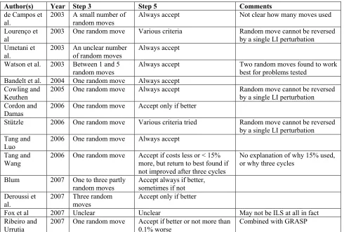
Table 1 – Summary of some recently reported uses of Iterated Local Search

In addition, some authors have used slightly more complex variations of ILS. For example, Thierens (2004) and van der Vonder et al. (2007) use a population-based approach, while Zhang and Sun (2006) have incorporated an approach they call "guided mutation".

The aims of this paper

This paper, without claiming to give a definitive answer as to the best way to implement ILS (this would be much too ambitious for a single paper) therefore seeks to shed some light on this issue by means of an extensive set of experiments on a single problem. Using a single problem ensures that sufficient experimentation can be carried out to ensure very robust conclusions to be drawn for that problem, though of course they will need to be confirmed at a later date for other problems. The problem used is a complex and difficult one, in order to ensure good discrimination between methods, and is a real-life problem, ensuring practical relevance for any conclusions.

While in some respects the work may partly duplicate work already reported by other authors, there is an important respect in which it goes further. This is that the focus is on achieving as good a solution as possible within a predetermined amount of computational effort (defined as number of iterations rather than computer time for reasons of consistency, since the experiments were run on several computers under different conditions). Too often we see results reported which are very difficult to interpret because different approaches are allowed to run for different lengths of time, or numbers of iterations.

Author(s) Year Step 3 Step 5 Comments

de Campos et

al. 2003 A small number of random moves Always accept Not clear how many moves used

Lourenço et al

2003 One random move Various criteria Random move cannot be reversed

by a single LI perturbation Umetani et

al. 2003 An unclear number of random moves Always accept Watson et al. 2003 Between 1 and 5

random moves Always accept Two random moves found to work best for problems tested Bandelt et al. 2004 One random move Always accept

Cowling and

Keuthen 2005 One random move Always accept Random move cannot be reversed by a single LI perturbation Cordon and

Damas

2006 One random move Accept only if better

Stützle 2006 One random move Various criteria tried Random move cannot be reversed

by a single LI perturbation Tang and

Luo 2006 One random move Always accept

Tang and

Wang 2006 One random move Accept if costs less or < 15% more, but return to best found if not improved after three cycles

No explanation of why 15% used, or why three cycles

Blum 2007 One to three partly

random moves Accept always if better, sometimes if not Deroussi et

al. 2007 Three moves random Accept only if better

Fox et al 2007 Unclear Unclear May not be ILS at all in fact

Ribeiro and

Short runs and (fairly) long runs were both used to see whether any conclusions would depend on the length of a run – and indeed some of them did, which is probably the most interesting feature of the results. It is not intuitively surprising that the best strategy for any search procedure may depend upon the length of time, or number of iterations, available, but most previous research has not examined this in a direct way.

Another novel aspect of the work is that it considers variations which are applicable specifically for problems with many objectives, as well as to those with just one objective. This involves the "kick" stage, which was allowed to be partly non-random as well as maintaining a random element; the number of random and non-random moves in each kick formed part of the investigation. The way in which non-random moves were chosen was also examined; this used information about subcosts as well as the overall cost in the manner of Wright (2001).

In addition, it is important to avoid a search which keeps returning to the same local optimum. Some researchers, e.g. Stützle (2006), recommend that this should be done by making the "kick"

sufficiently complex that it can not be reversed by a single perturbation, but it seems more natural to use the same method as is used in Tabu Search – see Glover (1990) – which is to make such a reversal tabu for a certain length of time.

The experiments

The series of experiments reported here necessarily considers only fairly simple variations of ILS, implemented on a real-life scheduling problem with many objectives. This involved the scheduling of cricket umpires to a league – see Wright (2007) for fuller details. 52 umpires needed to be allocated to 135 matches on nine different dates subject to there being two umpires for every match and no umpire having more than one match on any given date. The number of objectives to be incorporated into the cost function was 13, involving the amount of work done at different levels by umpires, how often they were paired with each other, how often they encountered particular teams, travel distances, etc.

This problem was chosen because it is complex and difficult enough to present a challenging test for the methods implemented (otherwise there is a danger that the optimal solution may be frequently reached, which then reduces the discrimination between variations), while not being so large as to make rigorous experimentation impossible.

All of the experiments used initial solutions that were constrained to be feasible but which were otherwise entirely random, and the same LI procedure, a "first-found descent" method with

perturbations consisting of either the replacement of one umpire by another for a specific match or the swapping of two umpires between two matches. Perturbations were examined in a fixed order, being accepted if they decreased overall cost but rejected otherwise, and this was then repeated until all perturbations had been examined since the last change was accepted.

Possible "kicks" were defined in the same way as the perturbations for the local improvement, rather than n in a more complex manner as suggested by Stützle (2006). A reversal of a "kick" move was tabu for three loops through the set of possible perturbations, or until the next local optimum was reached, whichever came sooner. This ensured that successive local optima were almost certainly different.

For the first set of experiments, five parameters were varied:

• I, the number of iterations for each run – this was either 200,000 (short) or 2,000,000 (long).

To put these figures in context, the initial LI stage generally took between 25,000 and 30,000 iterations, while subsequent LIs took between about 3,000 and about 15,000 iterations, depending upon the "strength" of the kick. In fact, the stopping criterion was always invoked at the end of an LI, so that the number of iterations was always a little greater than I, but not so much as to affect the validity of any results.

• M, the number of random perturbations involved in each kick – these perturbations were of

the same type as those used in the LI stages of the search, and was set at 1, 2 or 3 (M = 0 was tried initially as well, but it soon became clear that this was producing vastly inferior

solutions, so this line of enquiry was not pursued further).

• N, the number of non-random perturbations involved in each kick – this varied between 0 and

8 for short runs and between 0 and 5 for long runs.

• η, a parameter relating to the way in which the non-random perturbations were selected (and

thus not required when N = 0). The perturbations were chosen which minimised (C – ηB),

where C is the increase in overall cost and B is the highest decrease in any single subcost (usually positive). This is an idea put forward by Wright (2001) which was shown to

improve solutions for certain problems. The following values of η were considered: 0, 0.25,

0.5, 1 and 2. Thus a combination of M = 0, N = 1 and η = 0 is equivalent to a simple form of

Tabu Search.

• κ, a parameter which determined the rules for acceptability of a new LO. κ denoted the

probability of accepting a new LO whose cost was worse than or equal to that of the previous

LO: an LO with lower cost was always accepted whatever the value of κ . The values used

for κ were 0 (a kind of meta-local-improvement), 1 (a kind of meta-random-walk) and 0.5

(something between). More complex acceptance rules were considered in the second set of experiments.

100 runs were made for each combination of parameter values. There were thus 36,900 short runs and 23,400 long runs, generating over 50 billion iterations, and producing over 60 thousand "best" solutions (the cost recorded for each run was the cost of the best solution encountered, not necessarily the final solution). It is possible that all of these best solutions were different – certainly the best of all was encountered only once, and it is not known whether it is an optimal solution.

Results of first set of experiments

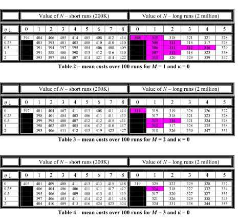
First we show the results for κ = 0, i.e. when a new local optimum is accepted if and only if its cost is

lower than the cost of the current local optimum. The mean costs for each combination of parameters are summarised briefly in Tables 2 to 4.

Value of N – short runs (200K) Value of N – long runs (2 million)

η↓ 0 1 2 3 4 5 6 7 8 0 1 2 3 4 5

0 394 404 406 405 414 405 408 412 414 308 315 318 321 321 328

0.25 403 393 401 403 408 410 410 410 309 311 318 317 328

0.5 391 394 397 395 404 406 408 409 306 311 312 316 329

1 391 388 400 398 413 412 416 410 307 312 318 323 338

2 393 397 404 407 414 421 414 422 313 320 329 339 347

Table 2 – mean costs over 100 runs for M = 1 and κ = 0

Value of N – short runs (200K) Value of N – long runs (2 million)

η↓ 0 1 2 3 4 5 6 7 8 0 1 2 3 4 5

0 397 401 404 407 411 413 408 411 414 311 319 319 326 326 327

0.25 398 401 404 403 406 411 411 413 317 318 321 323 328

0.5 399 395 400 407 412 412 415 411 313 316 321 324 328

1 398 402 405 405 416 412 410 417 312 317 328 335 338

2 393 406 411 412 413 419 423 427 318 326 330 347 353

Table 3 – mean costs over 100 runs for M = 2 and κ = 0

Value of N – short runs (200K) Value of N – long runs (2 million)

η↓ 0 1 2 3 4 5 6 7 8 0 1 2 3 4 5

0 403 401 409 408 411 413 413 415 418 319 325 323 329 328 337

0.25 406 404 406 406 411 411 417 412 314 318 327 332 334

0.5 395 406 406 409 408 413 411 413 317 320 327 327 335

1 397 406 403 411 414 412 411 418 321 326 329 338 343

2 404 410 409 413 416 424 423 424 324 331 338 344 355

Table 4 – mean costs over 100 runs for M = 3 and κ = 0

Next we show the results for κ = 0.5, i.e. when a new local optimum is accepted if it has lower cost

than the current local optimum, and is accepted with a probability of 50% otherwise. The mean costs for each combination of parameters are summarised briefly in Tables 5 to 7.

Value of N – short runs (200K) Value of N – long runs (2 million)

η↓ 0 1 2 3 4 5 6 7 8 0 1 2 3 4 5

0 403 412 410 410 404 409 408 408 402 322 320 320 326 321 325

0.25 398 398 401 405 397 397 404 398 321 315 322 321 322

0.5 397 392 391 392 398 397 399 393 313 317 317 319 317

1 390 391 393 390 392 398 394 405 313 315 321 321 322

2 391 392 397 397 400 404 406 410 320 323 327 335 339

Value of N – short runs (200K) Value of N – long runs (2 million)

η↓ 0 1 2 3 4 5 6 7 8 0 1 2 3 4 5

0 408 407 412 409 410 406 408 413 409 326 328 326 329 331 333

0.25 399 399 397 405 402 405 405 400 332 321 324 328 326

0.5 398 401 398 401 401 400 403 400 320 320 322 327 329

1 397 400 395 392 396 402 399 403 323 324 326 326 329

2 403 396 407 403 405 407 411 412 327 331 337 341 342

Table 6 – mean costs over 100 runs for M = 2 and κ = 0.5

Value of N – short runs (200K) Value of N – long runs (2 million)

η↓ 0 1 2 3 4 5 6 7 8 0 1 2 3 4 5

0 409 410 404 408 411 408 409 417 412 333 332 333 331 330 335

0.25 404 408 403 403 406 401 403 408 326 331 328 330 333

0.5 401 402 401 397 404 406 403 411 329 331 329 335 332

1 401 400 404 403 405 403 405 404 328 331 331 334 336

2 397 401 406 412 414 410 415 414 334 338 344 342 349

Table 7 – mean costs over 100 runs for M = 3 and κ = 0.5

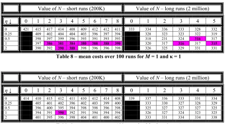
Finally we show the results for κ = 1, i.e. when every new local optimum is accepted. The mean costs

for each combination of parameters are summarised briefly in Tables 8 to 10.

Value of N – short runs (200K) Value of N – long runs (2 million)

η↓ 0 1 2 3 4 5 6 7 8 0 1 2 3 4 5

0 421 415 417 414 408 409 412 412 411 333 334 336 333 328 332

0.25 409 402 404 404 403 396 397 394 328 323 323 322 319

0.5 398 397 399 396 393 391 393 393 318 231 324 316 317

1 397 386 381 384 380 388 388 390 320 317 316 317 315

2 390 392 390 388 398 396 396 398 326 325 329 331 331

Table 8 – mean costs over 100 runs for M = 1 and κ = 1

Value of N – short runs (200K) Value of N – long runs (2 million)

η↓ 0 1 2 3 4 5 6 7 8 0 1 2 3 4 5

0 414 410 415 412 411 410 412 414 408 339 337 336 333 331 334

0.25 405 401 402 396 402 403 399 400 333 330 327 328 329

0.5 396 400 395 394 398 398 396 398 325 327 327 327 325

1 394 391 390 392 391 394 394 394 326 327 324 323 325

2 401 395 396 398 404 401 400 402 333 331 334 334 338

Value of N – short runs (200K) Value of N – long runs (2 million)

η↓ 0 1 2 3 4 5 6 7 8 0 1 2 3 4 5

0 414 417 413 411 410 407 412 413 403 342 342 339 337 339 339

0.25 410 406 405 400 405 404 407 402 336 333 332 331 336

0.5 404 402 398 396 400 399 406 405 335 331 333 329 333

1 401 397 394 395 393 396 395 403 334 330 329 333 337

2 400 398 396 401 402 402 405 405 335 339 339 342 346

Table 10 – mean costs over 100 runs for M = 3 and κ = 1

Standard deviations for the more successful combinations were mainly between 25 and 30 for the short runs, and between 15 and 25 for the long runs. Therefore means are significantly different at a level of more than 99% if they are apart by about 10 or more, using normality assumptions which appear to be reasonable. Results within 10 of the best mean found have therefore been highlighted in the tables.

Second set of experiments

The second set of experiments considered more complex forms of acceptance criterion, as follows.

• Simulated annealing (SA) method: a new local optimum was accepted if it was less costly

than the previous local optimum, otherwise it was accepted with a probability e – ∆C / T _{, where}

∆C is the increase in cost compared to the previous local optimum and T is a varying

temperature parameter. This uses the idea presented by Martin et al. (1996).

• Threshold acceptance (TA) method: a new local optimum was accepted if it was less costly

than the previous local optimum, otherwise it was accepted if and only if ∆C < T, where ∆C

is the increase in cost compared to the previous local optimum and T is a varying threshold parameter. This method is thus very similar to SA in nature except that it is deterministic. It accepts a new local optimum if and only if it would have been accepted under the SA method

with a probability in excess of e – 1 _{, i.e. about 0.37, using the same value of T.}

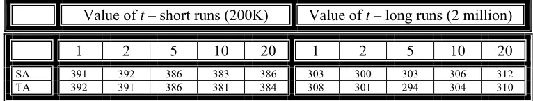
For each method, T decreased geometrically between a starting value of 10t and a finish value of t, where t = 1, 2, 5, 10 or 20.

Both short and long runs were carried out as before; however, for these experiments the other parameters were fixed at values that proved successful in the first set of experiments, i.e. N = 3, M =

1, η = 1 and κ = 1. The results are shown in Table 11.

Value of t – short runs (200K) Value of t – long runs (2 million)

1 2 5 10 20 1 2 5 10 20

SA 391 392 386 383 386 303 300 303 306 312 TA 392 391 386 381 384 308 301 294 304 310

Table 11 – mean costs over 100 runs for second set of experiments

more complicated criterion than either always accepting a new local optimum (κ = 1) or accepting it

only if it is better (κ = 0).

However, for the short runs, most of these results are only about the same as the best results from the

first set of experiments, which are achieved when κ = 0. Since a significant drawback of these more

complex methods is that the parameter t needs to be set (even though results are not very sensitive to

its value over a wide range), it is probably better for short runs just to use κ = 0.

Some very long runs, with 10 million iterations each, were also carried out:

1. 100 runs with N = 3, M = 1, η = 1 and κ = 0, i.e. only accepting better solutions

2. 100 runs with N = 3, M = 1, η = 1 and the simulated annealing acceptance criterion with

temperatures starting at 100 and ending at 10.

The results were not significantly different, averaging 281 and 282 respectively.

Conclusions

Putting together all the results, we can reach the following tentative conclusions. They have of course been shown to apply only for one instance of one type of problem; while it is reasonable to suppose that our conclusions may hold more widely, this can only be speculation until further experiments are carried out for other problems.

• M = 1 appears to work significantly better than M = 2 or 3; in other words, the kick should

only contain one random element. It may be, however, that if a tabu condition had not been included then there might have needed to be a little more randomness in the kick, or else the kick would have needed to be more complex, as suggested by Stützle (2006) and others.

• η = 0 is a relatively poor option, especially for short runs, and η = 0.5 or 1 is probably best;

maybe a value of 1 is overall slightly better than a value of 0.5. Thus, if the kick is to include a non-random element, the subcost-guided approach does appear to be valuable (obviously only for a problem with many subcosts).

• The results (perhaps surprisingly) are not very sensitive to the value of N when η > 0, though

perhaps values between 1 and 5 are best; so it is probably worthwhile to include some carefully selected non-random element in the kick.

• For short runs, a good approach is to set κ = 1 (accepting all new local optima), since it is at

least as good as other methods considered and has the merit of being simpler, without any need for tuning of parameters. This can perhaps be explained by the fact that short runs need

extra diversification which is supplied by accepting all new local optima. κ = 0 appears not

to do well in these circumstances, and κ = 0.5 falls between the two.

• For longer runs, where the very length of a run provides further diversification, the best tactic

appears to be to use a more complex acceptance criterion such as SA or TA. This however does have the drawback that the value of t needs to be tuned in advance, though the results

show that a very wide range of values of t will give good results. Otherwise κ = 0 (only

accepting better local optima) appears to work better than κ = 1 (always accepting), with

again κ = 0.5 falling between the two.

• For very long runs, it appears to be just as good to adopt the policy of only accepting better

local optima (κ = 0) as to employing a more complex technique such as Simulated Annealing.

• If η is constrained to be zero, as of course would be the case for a single-objective problem, N

= 0 is best; giving a wider interpretation to this, the results suggest that, if there is to be a non-random element to the kick, it should consist of something more than just choosing the perturbation(s) that increase cost by the least.

• If indeed η is constrained to be zero, it seems that κ = 0 works best, for both short and long

Overall, these results highlight the potential benefits to be drawn from treating short runs and long runs separately – the best policies may well be different.

The conclusions concerning the best conditions for a simulated annealing approach appear to back up the results of Marett and Wright (1996), who claimed that "the relative superiority of simulated annealing increases as the complexity of the combinatorial problem increases and as the number of perturbations allowed decreases".

Future research

These experiments need to be repeated for other problems to see whether or not similar conclusions hold. Other areas of potential interest could include:

• the effects of different acceptance criteria, including dynamic methods whereby the precise

criterion depends upon the progress of the search to date;

• the effects of different ways of choosing non-random elements of a kick – perhaps there

could be a dynamic element to this also;

• the relative effectiveness of using a simple random element with a tabu condition compared

with using a more complex random element without.

References

Bandelt H-J, Maas A and Spieksma FCR (2004) "Local search heuristics for multi-index assignment problems with decomposable costs", Journal of the Operational Research Society 55, 694–704

Blum C (2007) "Iterated local search and constructive heuristics for error correcting code design", International Journal of Innovative Computing and Applications 1(1), 14-22.

Cordon O and Damas S (2006) "Image registration with iterated local search", Journal of Heuristics 12, 73-94 Cowling PI and Keuthen R (2005) "Embedded local search approaches for routing optimization", Computers

and Operations Research 32(3), 465-490

de Campos LM, Fernández-Luna JM and Miguel Puerta J (2003) "An iterated local search algorithm for learning Bayesian networks with restarts based on conditional independence tests", International Journal of Intelligent Systems 18(2), 221-235

Deroussi L, Gourgand M and Tchernev N (2007) "A simple metaheuristic approach to the simultaneous scheduling of machines and automated guided vehicles", International Journal of Production Research

45(1), 1-22

Fox B, Xiang W and Lee HP (2007) "Industrial applications of the ant colony optimization algorithm",

International Journal of Advanced Manufacturing Technology 31, 805-814 Glover F (1990) "Tabu search: a tutorial", Interfaces 20(4), 74-94

Glover F (1995) "Tabu Thresholding: improved search by nonmonotonic trajectories" ORSA Journal on Computing 7(4), 426-442

Hoos HH and Stützle T (2005) Stochastic Local Search: Foundations and Applications, Elsevier, San Francisco, USA

Kelly JP, Golden BL and Assad AA (1993) "Large-scale controlled rounding using tabu search with strategic oscillation", Annals of Operations Research 41(2), 69-84

Lourenço HR, Martin OC and Stützle T (2003) "Iterated Local Search", in Handbook of Metaheuristics, eds. F Glover and EA Kochenberger, Kluwer, Boston, USA, 321-353

Marett RC and Wright MB (1996) "A comparison of neighbourhood search techniques for multi-objective combinatorial problems", Computers and Operations Research 23(5), 465-483

Martin O and Otto SW (1996) "Combining simulated annealing with local search heuristics", Annals of Operations Research 63, 57-75

Mladenović N and Hansen P (1997) "Variable Neighborhood Search", Computers and Operations Research 24, 1097-1100

Ribeiro CC and Urrutia S (2007) "Heuristics for the mirrored traveling tournament problem", European Journal of Operational Research 179(3), 775-787

Stützle T and Hoos HH (2002) "Analysing the run-time behaviour of iterated local search for the travelling salesman problem", in Essays and Surveys in Metaheuristics, eds. CC Ribeiro and P Hansen, Kluwer, Boston, USA, 589-611

Tang L and Luo J (2006) "A new ILS algorithm for parallel machine scheduling problems", Journal of Intelligent Manufacturing 17, 609-619

Tang L and Wang X (2006) "Iterated local search algorithm based on very large-scale neighbourhood for prize-collecting vehicle routing problem", International Journal of Advanced Manufacturing Technology 29, 1246-1258

Thierens D (2004) "Population-Based Iterated Local Search: Restricting Neighborhood Search by Crossover",

Lecture Notes in Computer Science 3103, 234-245

Umetani S, Yagiura M and Ibaraki T (2003) "One-dimensional cutting stock problem to minimize the number of different patterns", European Journal of Operational Research 146(2), 388-402

van der Vonder S, Ballestin F, Demeulemeester E and Herroelen W (2007) "Heuristic procedures for reactive project scheduling", Computers and Industrial Engineering 52(1), 11-28

Voudouris C and Tsang E (1998) "Guided local search and its application to the travelling salesman problem",

European Journal of Operational Research 113(2), 80-110

Watson JP, Howe AE and Whitley LD (2003) "An analysis of iterated local search for job-shop scheduling",

Proceedings of the Fifth Metaheuristics International Conference, Kyoto, Japan

Wright MB (1994) "Timetabling county cricket fixtures using a form of tabu search" Journal of the Operational Research Society 45(7), 758-770

Wright MB (2001) "Subcost-guided search – experiments with timetabling problems", Journal of Heuristics 7, 251-260.

Wright MB (2003) "An overview of neighbourhood search metaheuristics", Lancaster University Management School Working Paper LUMSWP2003/087

Wright MB (2007) "Case study: problem formulation and solution for a real-world sports scheduling problem",

Journal of the Operational Research Society 58 (4), 439–445.