Constraint based Distance Estimation in Ad hoc Wireless Sensor

in Ad-Hoc Wireless Sensor Networks

Urs Bischoff, Martin Strohbach, Mike Hazas, and Gerd Kortuem

Lancaster University, Lancaster LA1 4YW, UK

Abstract. We propose a lightweight localisation approach for support-ing distance and range queries in ad hoc wireless sensor networks. In con-trast to most previous localisation approaches we use a distance graph as spatial representation where edges between nodes are labelled with distance constraints. This approach has been carefully designed to sat-isfy the requirements of a concrete application scenario with respect to the spatial queries that need to be supported, the required accuracy of location information, and the capabilities of the target hardware. We show that this approach satisfies the accuracy requirements of the ex-ample application using simulations. We describe the implementation of the algorithms on wireless sensor nodes.

1

Introduction

Cooperative localisation algorithms play an important role for wireless sensor networks. In cooperative localisation, nodes work in a peer-to-peer manner to compute a map of the network using only the resources provided by the nodes themselves [1]. This makes cooperative algorithms especially suited for sensor network deployments that require true ad hoc localisation without external infrastructure.

The design of cooperative localisation algorithms requires a careful tradeoff betweenfidelity andcomplexity. Fidelity refers to quality of the computed result and includes precision and accuracy, as well as timeliness. Because measurements used as input to localisation algorithms are to some degree unreliable or inaccu-rate, node locations cannot be determined with absolute certainty. Complexity refers to the amount of resources consumed by an algorithm. In the wireless sensor network literature, complexity is most often considered in the context of energy efficiency and network use, although hardware, memory and time requirements are also important. Complexity is important because typical sensor network com-ponents possess very limited resources for processing and communication.

In this paper, we describe a novel approach to cooperative localisation that focuses on supporting distance and range queries, and trades fidelity against complexity. A distance query retrieves the distance between two given nodes, and arange query retrieves the IDs of nodes that are within a given distance from a given node. This approach has been carefully designed to satisfy the requirements of a concrete application scenario with respect to the accuracy

K. R¨omer, H. Karl, and F. Mattern (Eds.): EWSN 2006, LNCS 3868, pp. 54–68, 2006.

c

of location information, the spatial queries that need to be supported and the capabilities of the target hardware. Our approach can be characterized as in the following ways.

1. In contrast to most previous approaches we use a distance graph as spatial representation where edges between nodes are labelled with distance con-straints. Node coordinates (absolute or relative) are not represented. 2. The distance constraint of each edge is represented as an interval [a,b]

indi-cating that the distance between two nodes is at least a and at most b. The distance intervals are used for modelling uncertainty and localisation errors. 3. A constraint propagation algorithm is used to compute an overall consistent

distance graph.

The next section discusses the localisation requirements of our application scenario. Following that is a description of the spatial model and the cooper-ative algorithm. We then evaluate the accuracy of our approach for range and distance queries using simulations, and we describe the resource requirements of an implementation of the algorithm on a specific type of wireless sensor node. Fi-nally, we contrast our approach to some well-known algorithm in wireless sensor networks, and provide a comparative quantification of the computational and memory requirements of our algorithm.

2

Motivating Application Example

The application scenario that motivates this research is taken from the chemical industry work place in which safe handling and storage of chemical containers is of key importance. The goal here is to assist trained staff in detecting hazards of inappropriately stored chemicals. These hazards are defined by safety rules that are defined in terms of the storage conditions of the chemicals. For example, they prescribe that incompatible materials, such as reactive chemicals, must not be stored in immediate proximity. The meaning of “proximity” depends on a number of parameters including the type of involved chemicals.

We have developed a wireless sensor network for detecting possible safety hazards [2, 3]. Chemical containers are moved around quite frequently and may end up in a location without global networking capabilities, for example during transport inside the hull of ships or trucks. Moreover, it is generally unrealistic to rely on centralised services in environments that deal with chemical contain-ers. Thus the key design goal was to enable the detection of safety hazards without the involvement of external infrastructure. This required a cooperative approach in which the containers themselves are able to sense their environment and interpret their storage conditions with respect to predefined safety rules. We achieved this goal by embedding perception, safety rules and higher-level reasoning capabilities into sensor nodes attached to chemical containers.

2.1 Peer-to-Peer Position Sensing

mobile computing devices [4]. The simplified version does not require a connec-tion to a host PC and delivers accurate range informaconnec-tion between nodes of a wireless sensor network. Using the Relate technology we can directly measure the distance between co-located nodes and do not have to rely on network measure-ments such as received radio signal strength. The maximum distance that can be measured by Relate is about two meters. Relate nodes cooperate by broad-casting distance measurements over the network. Thus each node has access to distance measurements between a wide range of nodes and using the algorithm described in this paper can build a spatial model of its network neighbourhood.

2.2 Localisation Requirements

In our application scenario a containerA tries to detect whether there are any reactive chemicals in its proximity, whereby proximity is defined as a circular area aroundAwith a domain-specific radius. In this situationAneeds to deter-mine which containers are located within the proximity zone and which ones are located outside of it. The cooperative reasoning process described in [2] involves all nodes located within the proximity zone, regardless of their absolute loca-tion. Consequently, the spatial model for this application example must be able to support range queries, i.e. queries that return all nodes located in a specified range around a given node.

The required precision of the distance and range information depends in large measures on the physical dimensions of chemical containers. A chemical container as used in our application scenario is barrel-shaped and has a diameter between 60 and 80 cm. We assume that a range measurement precision of about half the diameter of a container is high enough. The Relate system provides measurements with 10 cm granularity or better, but only within the relatively short detection range of its ultrasound transducers (2 m). Thus a localisation algorithm must be able to indirectly compute distances between nodes that are beyond this range.

2.3 Hardware Requirements

The hardware used for instrumenting a chemical container is comparable to that used in other wireless sensor networks nodes such as the Berkeley Motes. The hardware consists of two separate components. The Relate component imple-ments peer-to-peer distance sensing, and the arteFACT component impleimple-ments the reasoning framework. Both are based on the Particle Smart-its, an embedded wireless sensing platform [5]. Particle Smart-Its incorporate a PIC 18F6720 mi-crocontroller with 128 KB of program flash memory and 4 KB of RAM. Particle Smart-its communicate via a slotted RF protocol and can provide effective data rates of up to 39 kbit/s. In the following we will describe the localisation system we designed for this application scenario.

3

Spatial Model and Algorithm

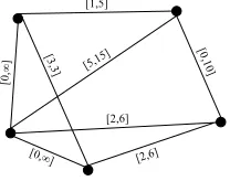
network nodes. Node coordinates (absolute or relative) are not represented. To represent constraints we use a graph where edges between nodes are labelled with distance intervals. More formally, adistance graphis an undirected labelled graphG= (N, E, C) whereN is a set of network nodes,E is a set edges andC is a constraint function which assigns to each edge adistance interval[u, v] with u, v∈IR andu≤v. Distance intervals are used to represent knowledge about the real-world distance between nodes. If the edge between nodes A and B is labelled with the intervalIAB = [u, v] and d(A, B) is the real-world distance betweenAandB, then:

ud(A, B)v . (1)

Thus an interval [u, v] indicates that the distance between the two respective network nodes is at leastuand at mostv. An interval [u, u] indicates that the distance is exactlyu. An interval [0,∞] is the most generic (or empty) constraint since it does not limit the distance between nodes in any meaningful way. An edge labelled with an empty constraint can be omitted from the graph without any loss of information. Figure 1 shows an example of a distance graph.

Fig. 1.Example distance graph

The algorithm for computing and updating the distance graph is a modi-fied Floyd-Warshall algorithm for computing all-pairs shortest paths. Instead of adding distances and selecting a minimum distance in each step, it infers and adds distance intervals.

1. Initialize all edges with the empty constraint [0,∞]

2. Receive distance measurements from Relate positioning system. 3. For all edges perform the modified Floyd-Warshall iteration:

(a) infer new distance interval, and

(b) combine interval with interval inferred in previous iteration. 4. Go to step 2

Fig. 2.Two intervals are used to infer a third one

step assuming the position ofA andB. For simplicity reasons we assume zero-length (i.e. u = v) intervals. The distances d(A, B) and d(B, C) are already known, either because they have been inferred in a previous step or because they represent measurements. d(A, C) must be inferred in this step. We know that C must lie on the circle with radiusd(B, C) and centreB. Hence we can represent all possible distances between A and C as [d(A, C_min), d(A, Cmax)]. Equations (2)-(4) illustrate the inference steps for the general case.

IAB= [u1, u2], IBC = [v1, v2]

⇒ IAC= [v1−u2, u2+v2] if u2v1. (2)

IAB= [u1, u2], IBC = [v1, v2]

⇒ IAC= [u1−v2, u2+v2] if v2u1. (3)

IAB= [u1, u2], IBC = [v1, v2]

⇒ IAC= [0, u2+v2] if IAB∩IBC =∅. (4)

These inference steps for all interval cases are also illustrated in Fig. 3. If the dis-tance intervalsIAB between A and B andIBC between B and C do not overlap all nodes have a different position. Hence,d(A, C)>0 and the interval bound-aries are calculated according to case (a) (cf. (2)) and (b) (cf. (3)) respectively. Otherwise A and C could have the same position and the minimum distance is chosen to be 0 in the inferred interval (c) (cf. (4)). There could exist several paths between pairs of nodes. In the second iteration step the inferred interval I_{inf is therefore compared to the previously inferred interval}Ipre to obtain the smallest consistent interval Inew. Consistency means that there is a position for each node in the graph so that all calculated distances would lie in their respective intervals. Thus, if the graph is consistent before the Floyd-Warshall iteration step, the intervals in step 3b will overlap and the smallest consistent

interval is obtained by intersecting them (6). Otherwise, we create a consistent graph by choosing the smallest interval that contains both input intervals (5).

Ipre = [u1, v1] and I_{inf = [}u2, v2]

IF ((v1u2) OR (v2u1))⇒Inew = [min(u1, u2), max(v1, v2)] (5)

ELSE⇒Inew = [max(u1, u2), min(v1, v2)]. (6)

4

Evaluation

In this section we evaluate the feasibility and accuracy of our algorithm and spatial model. Using a simulation environment, we characterise the algorithm results in terms of range query success and in terms of distance accuracy. We also show that our algorithm can be implemented on a resource-constrained wireless sensing platform such as the Particle Smart-Its.

4.1 Accuracy

Accuracy was evaluated in a simulation environment. For the purposes of com-parison, our simulation parameters were similar to that described by Shang and Ruml [6].1_{Our test networks consist of two hundred sensor nodes. The nodes are}

randomly placed, using a uniform distribution, within a 10r×10rsquare area. Next, a measurement range is chosen; our standard range is 2r. Each node can measure the distance to neighbouring nodes that are within the measurement range. These distance measurements build the input to our inference algorithm. A single experiment simulates one hundred random networks each consisting of two hundred nodes.

In early experiments, we used an error model for modelling measurements more realistically. The error model was based on experiments with Relate USB dongles [4] that have similar characteristics as the Relate devices we used. In one experiment it was shown that 90% of the true distances lie in the interval [d− 2cm,d+4.5cm]; dis the measured distance. However, tests showed that the error model does not have a big influence on the final errors. It is the algorithm itself that introduces the biggest errors; so the influence of the initial measurement errors and interval lengths is negligible for the overall end result.

Thus, we decided not to use this error model. This allows us to produce results that are more easily comparable to other algorithms because they are indepen-dent of the underlying error model which is based on a specific technology. In the following we present the evaluation results of these experiments.

1

Despite this, the results of our algorithm cannot be directly compared to that of

0.700 0.75 0.80 0.85 0.90 0.95 1.00 10

20 30 40 50 60 70 80

Interval (mapped onto [0,1])

Percentage of real distances

1.2r (8.1) 1.5r (12.3) 2.0r (20.8) 2.5r (31.1)

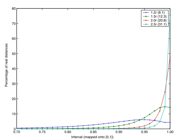
Fig. 4.Distribution of distances within intervals. As shown, this distribution depends on the measurement radius (connectivity).

We first analysed the characteristics of the intervals. As mentioned earlier the algorithm computes intervals; hence, if we want to do range queries, a position within each interval has to be chosen as the represented distance of the inter-val. We observed that the ground truth distances are not uniformly distributed within the intervals produced by our algorithm. We projected all intervals onto a standard interval [0,1]. These intervals were subdivided into one hundred subin-tervals. Then, we counted the number of times a real distance falls within the limits of each of the hundred sub-intervals; Fig. 4 shows that most real distances are close to the upper boundary of the interval results.

There are two main reasons for this. It can be shown that the lower boundary decreases faster than the upper boundary increases with each inference step. So, it is more probable that the real distance is not around the centre of the interval but closer to the upper boundary. This effect is intensified if several steps are necessary to infer the distance interval to another node. Because distant nodes are in the majority, we can clearly see this tendency in the overall distribution. There is also a geometric explanation. In Fig. 2, we showed that A sees C as lying on a circle around B. If we assume that the position of C is uniformly distributed on the periphery of the circle, we can see that the distanceAC is not uniformly distributed betweenAC_{min and}ACmax; the probability density is higher toward the boundaries.

We have experimented with various interval positions and measurement ranges. An optimal choice ofpdepends, among other reasons, on the connectivity of the graph. Because we do not know the connectivity in advance, we have to find a good trade-off. We chose the interval positionp= 0.98 for our next experiments that are based on different sets of simulated networks.

IAB= [u, v] ⇒ d(A, B)≈v−p(v−u) with p ∈[0,1]. (7)

Range Query Classification Error. In our range query scenario we are in-terested in the number of miss classifications. Therefore we distinguish between false positives and false negatives to characterize the accuracy of our algorithm. If a range query classifies a node as being inside the range even though it is out-side, it is a false positive. On the other hand, a false negative is a node reported to be outside the query range even though it is inside in reality.

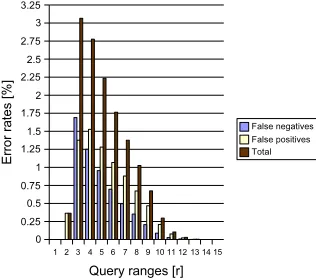
Figure 5 shows the error rate of false negatives, false positives and the total error as percentage of the number of nodes classified as being inside the respective circular query range. The measurement range is chosen to be 2r. The error rate is displayed with respect to the range specified in the query. Figure 6 depicts the same error but as percentages of the total number of nodes. The maximum false positive error ratio is 1.5% with respect to the number of nodes classified inside the query range. So for a query range of 4r, 1.5% of the nodes are wrongly classified as being inside the query range. With respect to the total number of nodes we have a maximum of 0.65% false positives, 0.45% of false negatives and a maximum total error of 1.1%.

For small ranges we have direct ultrasound distance measurements. For larger query ranges we depend on inferred distances. In both graphs we can therefore see an increase of the error rate at the beginning. Then, we observe a sharp decrease of the error rate. This is not because distance estimation is more accurate at

Fig. 5. Error rates in random uniform networks with respect to the number of nodes classified as being inside the range. The measurement range is 2r.

longer distances, but because we display classification errors as relative ones. For example, in Fig. 5 we show the error with respect to the total number of nodes classified inside the respective query range. So if the query range is increased and the absolute error remains the same, the relative error would decrease because of a larger number of nodes inside the query range. Similarly, in Fig. 6, for large query radii, most nodes clearly contain most of the other nodes in their range. Thus the probability of a misclassification is smaller. The maximum possible query radius of around 14r affects only a few nodes in the corners of the 10r×10rsquare area.

The previous test was based on a uniformly distributed random network. We expect our algorithm to perform worse if the shortest path distance between two nodes is long compared to the Euclidean distance. This is the case for nodes in the two wings of a C-shaped network. These networks consist of 160 nodes randomly positioned in C-shape; they are generated analogously to the random C-shaped placement used in experiments by Shang and Ruml [6].

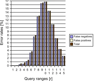
As expected we observe a higher error rate for the C-shaped network. Figures 7 and 8 show the classification error rates. The error rate is significantly higher. We observe a lot of false negative errors; the discrepancy between the Euclidean distance and the graph distance is the main reason for this. The error rate could be reduced by changing the value ofpin (7); the optimalpis topology-dependent. But because we do normally not know the topology in advance, we used the same pas in the experiments with uniform networks.

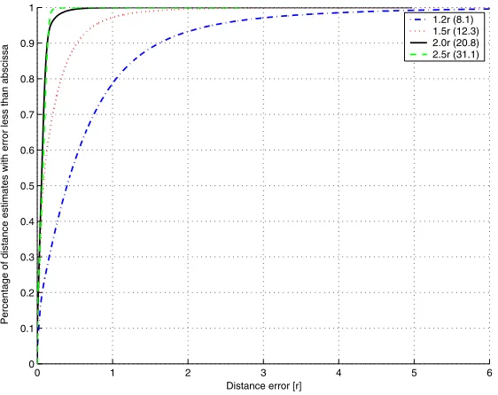
Distance Error. In order compare with other algorithms, we analysed the distance errors. Again we chose p = 0.98 as the distance position inside the intervals. Figure 9 shows a cumulative distribution of all the distance errors in the random uniform networks. In total, almost two million distances were represented in our simulations (100 networks consisting of 200 nodes each). All of these distances were compared with the inferred distances. Figure 9 shows,

Fig. 7.Error rates in random C-shaped networks with respect to the number of nodes classified as being inside the range. The measurement range is 2r.

0 1 2 3 4 5 6 0

0.1 0.2 0.3 0.4 0.5 0.6 0.7 0.8 0.9 1

Distance error [r]

Percentage of distance estimates with error less than abscissa

1.2r (8.1) 1.5r (12.3) 2.0r (20.8) 2.5r (31.1)

Fig. 9. Cumulative distribution of distance errors for p = 0.98 in random uniform topology. The distribution is shown for different measurement ranges (connectivities).

for example, that around 90% of the distances are less than 1.5r away from the real distance if we take 1.2r as our measurement radius. It is expected that the accuracy is improved if the measurement range (and connectivity) is increased. In the evaluation of the missclassification error, we chose a measurement radius of 2r. For this radius we expect the distance error of 90% of the nodes to be less then 0.15r.

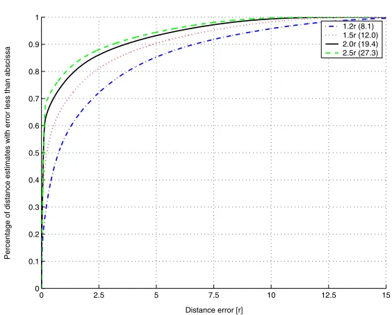
Figure 10 shows the cumulative distribution of distance errors in the ran-dom C-shaped networks. Although a large portion of the inferred distances are accurate, there is also a significant number of inferred distances that are not. Again the discrepancy between the graph distance and the Euclidean distance explains this observation. However, we have this extreme discrepancy between some pairs of nodes only. Shang and Ruml [6] only report the error medians, rather than their entire error distributions. However, our distance error median is comparable to their position error median.

4.2 Feasibility

The algorithm has been implemented on the Particle Smart-Its. The arteFACT component listens to measurement broadcasts by Relate nodes and maintains its own spatial model. The location model is updated by each node independently whenever a Relate node broadcasts its measurement updates.

0 2.5 5 7.5 10 12.5 15 0

0.1 0.2 0.3 0.4 0.5 0.6 0.7 0.8 0.9 1

Distance error [r]

Percentage of distance estimates with error less than abscissa

1.2r (8.1) 1.5r (12.0) 2.0r (19.4) 2.5r (27.3)

Fig. 10.Cumulative distribution of distance errors for p= 0.98 in random C-shaped topology. The distribution is shown for different measurement ranges (connectivities).

intervals to account for the case when devices have moved out of the ultrasound measurement range. This is achieved by timestamping the measurements with the local clock on arrival. In our prototypical implementation we chose a timeout of about 8s. Further experiments will help to choose this parameter according to update requirements. This will also help us to minimize the number of model up-dates for a given required update rate. Currently we update the model whenever we receive new measurements.

The current implementation supports a network of 10 nodes using 17% of the program memory and 64% of the data memory in the worst case. These are promising results, especially in the light that further optimizations are possible. For example, we use a fulln×nadjacency matrix to represent the graph.

5

Discussion

we do not have any false negatives, but only false positives (neglecting raw mea-surement errors). There is an optimalpthat minimises the overall error; the goal is to find a good trade-off between false positives and false negatives. However, if the application is very sensitive to only one kind of error, that kind of error could be minimised. We achieved a relatively low error rate for our range queries by ex-ploiting the non-uniform distribution of distances within the intervals.

Irrespective of the number of false positives and false negatives we also showed that the distance errors are small for most of the node pairs. In Sect. 2.2 we stated that the distance accuracy requirements of our application are around 30-40 cm. We showed for a measurement range of 2rthat the distance error of 90% of the nodes is less than 0.15r. So if we chooserto be around 1 m (which corresponds to the Relate measurement range of 2 m (= 2r)), we expect to satisfy these requirements. We first evaluated our algorithm on random uniform networks. We assume that these random networks did not represent the worst or best case. The perfor-mance of our algorithm is expected to be worse if the Euclidean distance between two nodes is small but a large number of inference steps are necessary to infer the distance interval, i.e. long graph distance between nodes. We modelled this scenario in random C-shaped networks.

For our scenario we have not exploited all the information. We do not directly make use of the fuzzy information that is given by the intervals. The length of the intervals could be an indicator for accuracy; we expect less accurate results if the intervals are longer.

The main advantage of our approach is its low complexity. We showed that it can be implemented on resource constrained embedded sensor nodes. Based on the requirements of our scenario, the algorithm only computes distances. This is in contrast to other location algorithms for wireless sensor networks which generally compute positions (cf. Sect. 6).

6

Related Work

We are not aware of any practical work on range queries in wireless sensor networks. However, there are several research areas that provide theoretical and practical foundations for our work. Hightower and Borriello provide a good overview of positioning systems for ubiquitous computing [7], and there have been a number of surveys describing and classifying positioning algo-rithms [8–10].

Most important to our work is the Relate project from which we used the sensing hardware. A USB dongle variant was used in [4] to provide relative positioning support for mobile devices. In contrast to our work, Relate dongles rely on host devices such as laptops or PDAs to compute the spatial model.

Com-pared to other methods the feasibility of their approach was demonstrated by implementing the algorithm on real sensor nodes. However, their technique can-not be directly applied to Cooperative Artefact networks as it relies on anchor nodes which have knowledge of their surveyed locations.

There exist a lot of localisation algorithms for wireless sensor networks. Most algorithms depend on anchor nodes because they compute absolute node posi-tions. Our application cannot depend on anchor nodes. Therefore, we mainly con-sidered relative positioning algorithms: MDS-MAP [12] and the Self-Positioning Algorithm (SPA) [13] are two typical examples, which calculate relative positions using simple connectivity. MDS-MAP uses an all-pairs shortest path algorithm to compute a distance matrix. Then, multi-dimensional scaling (MDS) is applied to find an embedding in the two-dimensional space. In SPA each node forwards dis-tance measurements to neighbouring nodes and calculates node positions using trigonometry in the local neighbourhood. Then, these local coordinate systems are merged into one coordinate system.

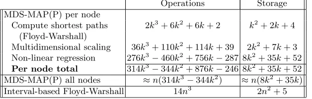
MDS-MAP(P) is an improved MDS-MAP algorithm [6]. It is a distributed lo-calisation algorithm which yields median accuracies similar to our algorithm. Table 1 shows the complexity of our algorithm, compared to that of MDS-MAP(P). To compute the complexity of MDS-MAP(P), we used the Numer-ical Recipes in C algorithms for eigenvector decomposition, and Levenberg-Marquardt non-linear regression.2 The step which merges the local maps, as well as some of the preprocessing steps in the eigenvector decomposition were neglected. In the per node computations which deal only with local maps, it was assumed that distance measurements were available for half the total pairs of neighbours. It was also assumed that the regression takes five iterations to complete.3

One of the advantages of the MDS-MAP(P) algorithm is that it is distributed. However, this means thateach node must first compute its own local map, and then work together with the other nodes to arrive at the global map. Assum-ing each node has the ten or more neighbours necessary to achieve reasonable accuracy, our interval-based Floyd-Warshall algorithm has lower processing re-quirements for networks with a total of one hundred nodes or less. It is also important to note that our interval-based Floyd-Warshall algorithm uses only 16-bit integer operations, whereas the MDS-MAP(P) steps mostly rely on float-ing point operations (such as computfloat-ing matrix inverses).

2

Because of the nature of location models where distances are related to (x, y) coor-dinates using the Euclidean relationship, the gradient matrix used by the regression algorithm holds only four non-zero gradients. Using this knowledge, large computa-tional savings (O(k3) instead ofO(k4)) can be made in the Levenberg-Marquardt al-gorithm. In our computations, we assumed that this optimisation had been made. To compute the complexity of the matrix inverse operations required by the

Levenberg-Marquardt method, we usedNumerical RecipesGauss-Jordan elimination with full

pivoting.

3

Table 1.Resource requirements of MDS-MAP(P) and interval-based Floyd-Warshall.

nis the total number of nodes in the network, andk is the number of neighbours to

each node.

Operations Storage

MDS-MAP(P) per node

Compute shortest paths 2k3_{+ 6k}2_{+ 6k+ 2 k}2_{+ 2k+ 4}

(Floyd-Warshall)

Multidimensional scaling 36k3_{+ 110k}2_{+ 114k+ 39 2k}2_{+ 7k+ 3}

Non-linear regression 276k3−460k2+ 756k−287 8k2+ 35k+ 52

Per node total 314k3−344k2+ 876k−246 8k2+ 35k+ 52

MDS-MAP(P) all nodes ≈n(314k3_−344k2_{) ≈n(8k}2_{+ 35k)}

Interval-based Floyd-Warshall 14n3 _2n2_{+ 5}

Thus, the MDS-MAP(P) algorithm trades off higher computational complex-ity and storage requirements in order to producecoordinate location results. By contrast, our algorithm requires less processing and storage, and instead esti-mates the node-to-nodedistances.

7

Conclusions

We have presented a lightweight localisation algorithm for ad hoc sensor net-works. The algorithm has been designed to satisfy concrete application require-ments in terms of the accuracy of location information, spatial queries and the capabilities of the target hardware. In contrast to most previous localisation ap-proaches our algorithm computes constraints on the distance between network nodes in the form of distance intervals. These intervals can be used to represent inaccuracy of distance measurements as well as imprecision as result of inference steps. The length of intervals can be seen as a quality measure for spatial infor-mation. In future work we will look at ways to improve the information quality by reducing the interval length. In particular, we are considering combining our approach with Freksa’s reasoning method for inferring spatial relations between neighbouring point objects in 2D [14].

References

1. Patwari, N., Ash, J.N., Kyperountas, S., III, A.O.H., Moses, R.L., Correal, N.S.: Locating the nodes: Cooperative localization in wireless sensor networks. IEEE

Signal Processing Magazine22(4) (2005) 54–69

2. Strohbach, M., Gellersen, H.W., Kortuem, G., Kray, C.: Cooperative artefacts: Assessing real world situations with embedded technology. In: Proceedings of the Sixth International Conference on Ubiquitous Computing (UbiComp). (2004) 3. Strohbach, M., Kortuem, G., Gellersen, H.W., Kray, C.: Using cooperative

4. Hazas, M., Kray, C., Gellersen, H., Agbota, H., Kortuem, G., Krohn, A.: A relative positioning system for co-located mobile devices. In: Proceedings of the Third International Conference on Mobile Systems, Applications, and Services (MobiSys). (2005)

5. TecO: Particle webpage.http://particle.teco.edu/devices/index.html(2005)

6. Shang, Y., Ruml, W.: Improved MDS-based localization. In: Proceedings of the 23rd Conference of the IEEE Communications Society (Infocom 2004). (2004) 7. Hightower, J., Borriello, G.: A survey and taxonomy of location systems for

ubiq-uitous computing. Extended paper from Computer 34(8) p57-66 (2001)

8. Langendoen, K., Reijers, N.: Distributed localization in wireless sensor networks:

A quantitative comparison. Computer Networks43(4) (2003) 499–518

9. Muthukrishnan, K., Lijding, M., Havinga, P.: Towards smart surroundings: En-abling techniques and technologies for localization. In: Proceedings of the First International Workshop on Location– and Context-Awareness (LoCA), Springer-Verlag (2005)

10. Niculescu, D.: Positioning in ad hoc sensor networks. IEEE Network18(4) (2004)

24–29

11. Minami, M., Fukuju, Y., Hirasawa, K., Yokoyama, S., Mizumachi, M., Morikawa, H., Aoyama, T.: Dolphin: A practical approach for implementing a fully distributed indoor ultrasonic positioning system. In: Proceedings of the Sixth International Conference on Ubiquitous Computing (UbiComp). (2004)

12. Shang, Y., Ruml, W., Zhang, Y., Fromherz, M.P.J.: Localization from mere con-nectivity. In: Proceedings of the Fourth ACM International Symposium on Mobile Ad hoc Networking and Computing (MobiHoc), ACM Press (2003) 201–212 13. Capkun, S., Hamdi, M., Hubaux, J.: GPS-free positioning in mobile ad-hoc