Bootstrapping long memory tests: some Monte Carlo results

(1)

Lancaster University Management School

Working Paper

2006/002

Bootstrapping long memory tests: some Monte Carlo results

Anthony Murphy and Marwan Izzeldin

The Department of Economics

Lancaster University Management School

Lancaster LA1 4YX

UK

provided that full acknowledgement is given.

(2)

Bootstrapping Long Memory Tests: Some Monte Carlo Results

Anthony Murphy1

Department of Economics, University of Oxford

Marwan Izzeldin

Lancaster University Management School

August 2007

Abstract: We investigate the bootstrapped size and power properties of five common

long memory tests - the modified R/S, KPSS, V/S, GPH and Robinson’s _H_tests.

Even in samples of size 100, the moving block bootstrap controls the empirical size of

the tests in the DGPs examined. The H test appears to be the most powerful.

Moreover, the bootstrapped tests suffer little loss of power against fractionally

integrated processes vis á vis asymptotic tests with samples of 250 or more

observations. This is true both for distributions with heavy tails and with stochastic

volatility (SV).

Keywords: Moving block bootstrap, long memory, fractional integration.

JEL Code: C10, C12

(3)

1. Introduction

Long memory processes, especially fractionally integrated processes, describe

many financial time series as well as some macroeconomic series rather well. It is

important to distinguish long memory processes from more common I(0) and I(1)

processes as they imply different long run predictions and responses to shocks

(Baillie, 1996). A range of tests for long memory are available. Unfortunately, the

evidence is that tests based on asymptotic critical values are often badly sized.

In this paper we report the results of a series of Monte Carlo experiments used

to examine the size and power properties of five, commonly used, long memory tests

using asymptotic and bootstrapped critical values. The five tests are Lo's modified

rescaled range or R/S statistic (Lo, 1991), the KPSS statistic (Kwiatkowski et al.,

1992), the rescaled variance or V/S statistic (Giraitis et al., 2003), the GPH statistic

(Geweke and Porter-Hudak, 1983) and the H statistic in Robinson (1995) and

Robinson and Henry (1999). The set of tests considered is broader than in other

papers.

We use the moving block bootstrap (MBB) to mimic the dependence in the

data. All the test statistics are asymptotically pivotal. This means that, for dependent

stationary data satisfying reasonable regularity conditions, bootstrapped critical values

should provide a higher order of accuracy than asymptotic critical values. We found

this when we used the post-blackened MBB to examine the size and power of the

modified R/S statistic (Izzeldin and Murphy, 2000).

For the data generation processes we consider, we find that we can control the

size of all five tests using the moving block bootstrap even in small samples with as

few as 100 observations. We also find that bootstrapped tests suffer little loss of

power against fractionally integrated (FI) processes vis á vis asymptotic tests with

(4)

tails (log-normal random errors) and with stochastic volatility (SV). We also show

that all of the tests lack power against a particular type of fractionally integrated

process, the sum of a FI and a SV process as opposed to a FI process with a SV error.

The outline of this paper is as follows. We discuss the five tests of long

memory in next section. We briefly review the relevant empirical literature on the size

and power of these tests, as well as bootstrapped long memory tests, in Section 3. We

discuss the moving block bootstrap in Section 4 and discuss the Monte Carlo

experiments and our findings in Sections 5 and 6. We present a financial application

in Section 7 and conclude in Section 8.

2. Tests of Long Memory

We consider five tests of long memory – the modified rescaled range or R/S

statistic, the KPSS statistic, the rescaled variance or V/S statistic, the GPH statistic

and the _H_{statistic. The modified R/S, KPSS and V/S statistics for a time series {}

t x }

may be expressed in term of the partial sum of the standardized series

(

)

1

( ) t ( ) /

T _s s

S t =

∑

₌ x −x Tσ∞ , where 1 T₁ _t

t

x x

T =

=

∑

is the sample mean, _σ2∞ is an

estimate of the long run variance of { }x_t and Tis the sample size. Then:

1/ 2

0 0

/ max ( ) min ( )

t T t T

T− R S S t S t

≤ ≤ ≤ ≤

= − (1)

2 1 1 ( ) T T t

KPSS S t

T =

=

∑

(2)

2

1

/ T ( ( )_T T)

t

V S S t S

T =

=

∑

− (3)

When {xt} is stationary and under suitable regularity conditions:

1/ 2

1 ₀ ₁ 1 0 1

/ max ( ) min ( )

r r

T− R S W r W r

≤ ≤ ≤ ≤

(5)

1 ₂ 1 0 ( )

KPSS⇒

∫

W r dr (5)

(

)

2

1 ₂ 1 ₂

1 1

0 0

/ ( ) ( )

V S⇒

∫

W r dr−

∫

W r dr (6)

where ⇒ denotes convergence in distribution, W r₁( )=W r( )−rW(1) is a standard

first order Brownian bridge process and W r( ) is a standard Brownian motion

process.

Giraitis et al. (2003), inter alia, derive the asymptotic distribution of the R/S,

KPSS and V/S statistics under short and long memory assumptions. All three tests are

consistent against fractionally integrated alternatives. In addition, all three tests are

asymptotically pivotal, so appropriate bootstrap critical values should outperform

asymptotic critical values in smaller samples.

Geweke and Porter-Hudak (1983) show how to consistently estimate the

fractional integration parameter d in an ARFIMA model using a semi-nonparametric,

frequency domain procedure and derived its asymptotic distribution. For frequencies

near zero, d can be estimated from the least squares regression:

2

ln( ( ))I w_j = −c dln{(4sin (w_j/ 2)}+η_j, j=1,...n (7)

where ( )I w_j is the periodogram of the {x_t} series at the n frequencies w_j =2π j T/ .

Often the setting n=[ T] is chosen, where [ ] denotes the integer part. With a proper

choice of n, the asymptotic distribution of d does not depend on either the order of the

ARMA process or on the distribution of the error term in the ARFIMA process {xt}.

Asymptotically d is normally distributed with varianceπ2/ 6.

Robinson (1995) derives a semi-parametric, frequency domain estimator of the

fractional integration parameter d which is closely related to the trimmed Whittle

estimator in Kunsch (1987). He refers to it as a Gaussian or local Whittle estimator.

(6)

weak conditions. Moreover, the asymptotic variance of this estimator is free of

unknown parameters. Robinson also shows that it dominates the Geweke and

Porter-Hudak (1983) estimator. Robinson and Henry (1999) show that, under weak

conditions, these results continue to hold under common forms of conditional

heteroscedasticity of both the long and short memory kind.

For the sort of long memory processes usually estimated using financial time

series data, the Sk ⌢

test of Harris, McCabe and Leybourne (2006) appears to have

fairly similar size and power properties to the _H_{test in Robinson (1995), so we have}

not examined its performance here.

3. A Review of Previous Monte Carlo Studies

In this section we briefly review some of the more recent Monte Carlo results

in the literature on testing long memory. Lee and Schmidt (1996) show that the power

of the KPSS test against basic fractionally integrated (FI) alternatives in sample sizes

ranging from 50 to 500 is comparable to that of the modified R/S test. However, they

argue that rather larger sample sizes, such as T = 500 or T = 1000, are required to

distinguish reliably between a long memory process and a short memory process with

comparable short-term autocorrelation. Their results show that both tests are sensitive

to the choice of lag truncation i.e. the number of covariance terms used to calculate

the long run variance σ2∞.

Hauser (1997) investigates the size and power properties of the GPH test, the

modified R/S test, a semi-parametric frequency domain test due to Robinson (1994)

and a test based on the trimmed Whittle likelihood (Kunsch, 1987), inter alia. He

examines IID, AR(1), MA(1), FI, ARFIMA, GARCH and IGARCH data generation

(7)

performs satisfactorily for all of the models considered. He suggests that the R/S

statistic is generally robust with the disadvantage of relatively small power. The

trimmed Whittle likelihood has high power in general and is robust except for large

short run effects.

Teverovsky et. al. (1999) also show that the value of Lo's (1991) modified R/S

statistic is sensitive to the choice of the truncation lag used to estimate_σ2∞. As the

truncation lag increases, the test statistic has a strong bias towards accepting the null

of no long run dependence, even when the DGP is a basic FI process.

Giraitis et. al. (2003) examined the size and power of the modified R/S, KPSS

and V/S statistics using sample sizes of 500 and 1000 using AR(1), FI and long and

short memory linear ARCH (Robinson, 1991) DGPs. They find that the V/S statistic

achieves a somewhat better balance of size and power than the R/S and KPSS test.

They also highlight the sensitivity of the test to the choice of the truncation lag when

estimatingσ2∞.

Robinson and Henry (1999) report an extensive range of Monte Carlo results.

They consider IID, ARCH, FI, nearly integrated GARCH, EGARCH and long

memory linear ARCH models and three sample sizes (T = 64, 128 and 256). Their

estimator _H_{= −}_dɵ _{1/ 2}_{appears to perform reasonably well except in the nearly}

integrated GARCH case.

We now consider Monte Carlo studies using bootstrap methods. Hiemstra and

Jones (1997) use the original non-parametric bootstrap of Efron (1979), designed for

IID observations, to test for long memory in stock returns using the modified R/S

statistic. Anderson and Gredenhoff (1998) use the AR-sieve bootstrap in a Monte

Carlo experiment looking at the size and power of the modified R/S and GPH tests, as

(8)

integration using sample sizes of 750 and 1000 observations. They use four bootstrap

resampling procedures. Their basic sieve or residual based bootstrap involves re

-sampling (with replacement) the residuals from an estimated AR model, the maximal

order of which is selected using the Bayesian information criterion of Schwartz

(1978). They extend this procedure to incorporate ARCH(1) dependence in the

residuals. They find that the sieve bootstrap works well in controlling the size of the

tests.

Izzeldin and Murphy (2000) use the post-blackened moving block bootstrap to

examine the size and power of the modified R/S statistic. They consider IID, AR(1),

MA(1), ARCH(1), GARCH(1,1), MA(1) plus GARCH(1,1) and fractionally

integrated data generation processes with both normal and log-normal random errors.

The post-blackened MBB works well. Compared to the asymptotic critical values in

Lo (1991), the MBB controls the empirical size of the test well without reducing the

power against FI alternatives much.

De Peretti (2003) examines the size and power of the R/S, modified R/S, GPH

and two other test statistics using an AR model to pre-whiten the data and various

parametric and non-parametric bootstrap procedures. He does not use the MBB. He

presents his results using a variety of P value plots and size-power curves using AR(p)

and FI DGPs. He suggests that the proposed bootstrap procedure controls the

empirical size of the various tests reasonably well without any loss of power.

Finally, Grau-Carles (2005) follows Izzeldin and Murphy (2000) and uses the

post-blackened moving block bootstrap to examine the size and power of the R/S,

modified R/S, Robinson’s _H_{and one other test of long memory. He looks at}

relatively small samples (T = 100 and 300) and considers a range of DGPs - IID

uniform, normal and log-normal; AR(1) and MA(1); ARCH(1) and AR(1) plus

(9)

blackening MBB is generally good although the tests are not very powerful. However,

this may because he used a small block length of 5 for the MBB. In our Monte Carlo

experiments, the modified R/S test statistic, and to some extent the H statistic, is a

good deal more powerful than in Grau-Carles (2005).

4. The Moving Block Bootstrap

The two most common bootstrap procedures for time series are the moving

block bootstrap (MBB) and the AR-sieve bootstrap for stationary linear time series

(Buhlmann, 2002). Both procedures are easy to implement, at least in principle.

However the MBB bootstrap is the more general procedure so we use it in our Monte

Carlo experiments. In the most common version of the MBB, introduced by Kunsch

(1989) and Liu and Singh (1992), the bootstrap sample is obtained by resampling

fixed size blocks of observations rather than the individual observations themselves.

The blocks may overlap. We experiment with the post blackening bootstrap suggested

by Davison and Hinkley (1997), which combines the MBB and AR-sieve methods,

and obtained no better results than the ones reported below.

Of course, there are some practical and other problems with the MBB

(Maddala and Kim, 1998, p. 329-330). For example, the pseudo-time series generated

by the moving block method is not stationary even if the original series {x_t} is

stationary. The choice of block length may be problematic, so the cross-validation and

plug-in procedures in Hall, Horowitz and Jing (1995) and Lahirir, Furukawa and Lee

(2007), as well as the frequency domain bootstrapping procedures in Hidalgo (2003),

may be worth investigating. However, in practice, we did not find this to be the case.

(10)

5. The Monte Carlo Experiments

We consider a range of data generation processes (DGPs) in our Monte Carlo

experiments. Here we present representative results for five DGPs:- (i) the IID case;

(ii) the first order autoregressive AR(1) case; (iii) the AR(1) with stochastic volatility

(SV) case; (iv) the fractionally integrated (FI) case and (v) the fractionally integrated

(FI) with stochastic volatility (SV) case. These five cases seem relevant when

considering financial data.

In the AR(1) case, we set ρ = 0.5 which is definitely on the high side for

financial data. However if the MBB bootstrap works well with ρ = 0.5, it will also

work well when the level of autocorrelation is lower. Conditional heteroscedasticity is

common in financial data, so we consider a range of GARCH and SV DGPs. The two

DGPs generated similar results so we only present the SV results here.

The DGP in (iii) is _{(1 0.5 )}1

t t

x = − L − u where u_t =exp( / 2)h_t ε_t with

1

0.95

t t t

h = h₋ +η . The 0.95 coefficient on h_t₋₁ means that the SV conditional

heteroscedasticity is slow to decay. The random errors ε_t and η_t are mean zero,

independent normal random variables with variances equal to 1 10. For the

fractionally integrated DGPs, we set the FI parameter d equal to 1 3, a reasonable

value given the range of results in many empirical papers. In the case of (i), (ii) and

(iv), we look at normal and log normal random errors. We also consider to variants of

cases (iii) and (v) involving the sum of an AR(1) or FI process and a SV process

Many of the Monte Carlo results summarized in the previous section are based

on either rather large or quite small sample sizes. We use four sample sizes - T = 100,

(11)

or more observations are the norm in most economic applications. Much larger

sample sizes are common in financial applications.

The Monte Carlo results are based on 1000 replications. A 100 observation

"burn in" period is used. The bootstrap results are based on 999 bootstrap replications

using the moving block bootstrap with a block length of 10. In general, the results are

not sensitive to the choice of block length, as long as it is not too short.

The long-run variance σ2∞ in the R/S, KPSS and V/S statistics is calculated

using ₈4_T ₁₀₀

  estimated covariance terms - the midpoint of the two settings

considered by Lee and Schmidt (1999). We use the standard Newey and West (1987)

estimator of σ2∞. When calculating the GPH and H test statistics, we use _ T_

frequency domain terms. All the calculations are carried out in Ox (Doornik, 1999).

6. The Monte Carlo Results

The Monte Carlo results in Table 1 for the IID case show that, in line with

other results in the literature, the MBB is reasonably successful in controlling the size

of all five tests, especially in small samples (T = 100 or 250). This is true for both the

normal and heavy-tailed, lognormal error cases. The empirical and nominal sizes of

the asymptotic tests can differ quite a lot, especially for the modified R/S and H test

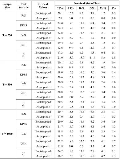
in small samples. Similar results are obtained in Table 2 using the AR(1) DGP.

We report the results for the AR(1) model with a stochastic volatility random

error term in Table 3. The SV random error with h_t =0.95h_t₋₁+η_t adds a slowly

decaying conditional heteroscedastic error, similar to a GARCH (1,1) error, to the

AR(1) model. The sizes of the asymptotic tests can be poor, whereas the nominal and

(12)

results are in line with the ARCH and GARCH results in Izzeldin and Murphy (2000)

and Grau-Carles (2005).

We report the power of the tests against the fractional integrated FI(d)

alternative, with d = 1/3, in Table 4. The power of the tests is higher when the

random error is log-normal than when it is normal. Unsurprisingly, the asymptotic

tests are generally more powerful than the bootstrapped tests, since we are reporting

power as opposed to size adjusted power. However, for moderate samples sizes (T ≥

250), the difference in power is generally small, the exception being the H test when

T = 250. When T ≥ 250, the power ranking of the bootstrapped tests appears to be _H_,

GPH, V/S followed jointly by the KPSS and the modified R/S tests. In smaller

samples, the power of all of the tests, apart from the asymptotic _H_{test, is low and the}

H test is not the most powerful one. Similar results are obtained for other values of d

in the range 0.1 to 0.4.

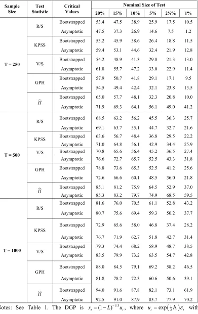
The power of the five tests against the FI alternative with a stochastic

volatility error term is set out in Table 5. The introduction of the SV error term only

results in a small reduction in power. The asymptotic tests are somewhat more

powerful when T = 250. The power ranking of the tests is much the same as in Table

4. The _H_{test is the most powerful, followed by either the GPH or V/S test.}

Finally we present some Monte Carlo results in Tables 6 for DGPs obtained

by summing an AR(1) or FI(d) process and a stochastic volatility process.

Unfortunately, in the FI-SV composite error case, none of the bootstrapped or

asymptotic tests has much power. In most cases, there is little difference in power

between the bootstrapped and asymptotic tests. The low power of the tests continues

to hold when, for example, h_t =0.5h_t₋₁+η_t is used to generate the SV component of

(13)

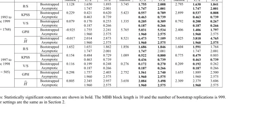
7. Financial Application

We apply the R/S, KPSS, V/S, GPH and _H_{long memory tests to daily}

Standard and Poor’s (SP500) returns, absolute returns and squared returns. We use the

data in Tsay (2005). We select the seven year sample period from January 1993 to

December 1999, a total of 1768 trading days. We also use a smaller, two year sample

from January 1997 to December 1998, a total of 505 days.

The long memory test results are shown in Table 7. Statistically significant

outcomes are shown in bold. In line with the literature, using the larger sample, we

cannot reject the null hypothesis of short memory in daily returns and we generally

reject the null hypothesis of short memory in absolute and squared daily returns.

However, in the smaller sample, we cannot always reject the null hypothesis of short

memory in the squared daily returns. These results are consistent with our Monte

Carlo results regarding the power of the tests.

In this example, the asymptotic and bootstrapped tests produce similar results.

However, even in the case of actual returns, the bootstrapped and asymptotic critical

values (and any corresponding P values) can differ quite a lot so it is worthwhile

bootstrapping the test statistics.

8. Summary and Conclusion

We use Monte Carlo methods to examine the size and power properties of five

widely used long memory tests – the modified R/S statistic, the KPSS statistic, the

rescaled variance or V/S statistic, the GPH statistic and Robinson’s H statistic. The

set of tests considered is broader than in other papers. We use the moving block

bootstrap to mimic the dependence in the data. All the test statistics are asymptotically

(14)

For all of the data generation processes we consider, we find that we can

control the size of all five tests using the moving block bootstrap even in small

samples with as few as 100 observations. We also find that bootstrapped tests suffer

little loss of power against fractionally integrated (FI) processes vis á vis asymptotic

tests with samples of 250 or more observations. This is true both for distributions with

heavy tails (log-normal random errors) and with stochastic volatility (SV). We also

show that all of the tests lack power against a particular type of fractionally integrated

(15)

References

Agiakloglou, C. and Newbold, P. (1994), “Lagrange Multiplier Tests for Fractional

Differences”, Journal of Time Series Analysis, 15(3), 253-262.

Andersen, M. and Gredenhoff, M. (1998), “Robust Testing for Fractional

Integration”, Working Paper 218 in Economics and Finance, Stockholm School of

Economics.

Baillie, R. T. (1996), “Long Memory Processes and Fractional Integration in

Econometrics”, Journal of Econometrics, 73, 5-59.

Buhlmann, P. (2002), “Bootstrap for Time Series”, Statistical Science, 17(1), 52-72.

Davison, A. C. and Hinkley, D. V. (1997), Bootstrap Methods and Their Application,

Cambridge University Press.

De Peretti, C. (2003), “Bilateral Bootstrap Tests for Long Memory: An Application to

the Silver Market”, Computational Economics, 22, 187-212.

Doornik, J. A. (1999), Object-Oriented Matrix Programming Using Ox, 3rd Edition,

Timberlake Consultants Press.

Efron, B. (1979), “Bootstrap Methods: Another Look at the Jackknife”, Annals of

Statistics, 7, 1-26.

Geweke, J. and Porter-Hudak, S. (1983), “The Estimation and Application of Long

Memory Time Series Models”, Journal of Time Series Analysis, 4(4), 221-238.

Giraitis, L., Kokoskva, P. Leipus, R. and Teyssire, G. (2003), “Rescaled Variance and

Related Tests for Long Memory in Volatility and Levels”, Journal of

Econometrics, 112(2), 265-294.

Grau-Carles, P. (2005), “Tests of Long memory: A Bootstrap Approach”,

Computational Economics, 25, 103-133.

Hall, P., Horowitz J. and Jing, B. (1995), “On Blocking Rules for the Bootstrap with

(16)

Harris, D., McCabe, B. and Leybourne, S. (2006), “Testing for Long Memory”,

Econometric Theory, forthcoming.

Hauser, M. (1997), “Semiparametric and Nonparametric Testing for Long Memory: A

Monte Carlo Study”, Empirical Economics, 22, 247-271.

Hidalgo, J. (2003), “An Alternative Bootstrap to Moving Blocks for Time Series

Regression Models”, Journal of Econometrics, 117, 369-399.

Hiemstra, C. and Jones, J. (2003), “Another Look at Long Memory in Common Stock

Returns”, Journal of Empirical Finance, 4(12), 373-401.

Hosking, J. (1981), “Fractional Differencing”, Biometrika, 68, 165-176.

Izzeldin, M. and A. Murphy (2000), “Bootstrapping the Small Sample Critical Values

of the Rescaled Range Statistic”, The Economic and Social Review, 31(4),

351-359.

Kunsch, H. R. (1987), “Statistical Aspects of Similar Processes”, in Prohorov, Y. and

Sazanon, V. V. (eds), Proceedings of the First World Congress of the Bernoulli

Society, VNU Science Press, Utrecht.

Kunsch, H. R. (1989), “The Jackknife and the Bootstrap for General Stationary

Observations”, Annals of Statistics, 17, 1217-1241.

Kwiatkowski, D., Phillips, P. C. B., Schmidt, P. and Shin, Y. (1992), “Testing the

Null Hypothesis of Stationarity Against the Alternative of a Unit Root: How Sure

are We That Economic Time Series Have a Unit Root?”, Journal of Econometrics,

54, 159-178.

Lahirir, S. N., Furukawa, K.and Lee, Y.-D. (2007), “A Non-Parametric Plug-In Rule

for Selecting Optimal Block Lengths for Block Bootstrap Methods”, Statistical

(17)

Lee, D. and Schmidt, P. (1996), “On the Power of the KPSS Test of Stationarity

against Fractionally-Integrated Alternatives”, Journal of Econometrics, 73,

285-302.

Liu, R. Y. and Singh, K. (1992), “Moving Block Bootstrap and Jackknife Capture

Weak Dependence”, in Le Page, R. and Billard, L. (eds), Exploring the Limits of

the Bootstrap, Wiley, NewYork.

Lo, A. (1991), “Long Term Memory in Stock Market Prices”, Econometrica, 59(5),

1297-1331.

Maddala, G. S. and Kim, I. M. (1998), Unit Roots, Cointegration and Structural

Change, Cambridge University Press, Cambridge.

Robinson, P. M. (1994), “Semiparametric Analysis of Long memory Time Series”,

The Annals of Statistics, 22, 515-539.

Robinson, P. M. (1995), “Gaussian Semiparametric Estimation of Long Range

Dependence”, The Annals of Statistics, 23, 1630-1661.

Robinson, P. M. and Henry, M. (1999), “Long and Short Memory Conditional

Heterskedasticity in Estimating the Memory Parameter of Levels”, Econometric

Theory, 15, 299-336.

Schwartz, G. (1978), “Estimating the Order of a Model”, The Annals of Statistics, 2,

461-464.

Teverovsky, V., Taqqu, M. and Willinger, W. (1999), “A Critical Look at Lo's

Modified R/S Statistic”, Journal of Statistical Planning and Inference, 80,

211-227.

(18)

17

Notes: The DGP is x_t =ε_t with ε_t _∼n i d. . (0,1) or, before demeaning, lnε_t _∼n i d. . (0,1). The Monte Carlo results are based on 1000 replications

using a 100 observation “burn-in” period. The bootstrap results are based on 999 bootstrap replications using the moving block bootstrap with a

block length of 10. The long run variance in the R/S, KPSS and V/S statistics is calculated using _[84_T_/100]_{estimated covariance terms. [√T]}

[image:18.612.59.718.76.413.2]

frequency domain terms are used to calculate the GPH and H test statistics.

Table 1: Size of Long Memory Tests for IID Models

Normal Random Error Demeaned Log-Normal Error Sample

Size

Test Statistic

Critical

Values _20% _15% _10% _5% _2½% _1% _20% _15% _10% _5% _2½% _1%

Bootstrapped 20.1 13.9 8.6 3.3 1.4 0.4 19.2 13.4 6.4 2.9 0.9 0.2

R/S

Asymptotic 7.1 2.8 0.4 0.1 0.0 0.0 4.3 1.5 0.2 0.0 0.0 0.0

Bootstrapped 21.2 15.8 10.4 5.0 3.3 1.2 22.1 16.3 10.4 5.1 2.6 1.1

KPSS

Asymptotic 21.7 15.3 9.4 3.8 1.0 0.0 23.4 16.7 10.0 2.8 1.10 0.0

Bootstrapped 20.5 14.7 8.5 3.4 1.4 0.5 20.3 14.2 8.7 4.9 2.0 0.7

V/S

Asymptotic 19.5 12.0 3.8 0.5 0.0 0.0 20.9 12.0 4.6 0.5 0.0 0.0

Bootstrapped 16.3 10.6 5.9 3.2 1.4 0.4 18.0 12.1 7.0 2.9 1.0 0.4

GPH

Asymptotic 6.7 5.5 3.7 1.5 0.7 0.2 8.9 6.8 2.9 1.3 0.3 0.3

Bootstrapped 13.5 8.5 5.5 2.6 1.0 0.1 15.6 10.1 5.3 2.1 0.6 0.1

T = 100

H

Asymptotic 16.3 13.1 10.4 6.9 5.0 3.2 16.9 14.8 10.9 7.1 5.0 2.4

Bootstrapped 21.1 15.0 10.3 5.4 3.4 1.2 19.2 13.5 8.5 4.3 2.2 0.5

R/S

Asymptotic 12.8 8.5 5.0 1.4 0.4 0.0 9.4 5.9 2.6 0.2 0.1 0.0

Bootstrapped 20.5 14.8 10.2 3.8 1.7 0.8 21.5 15.8 10.3 5.3 2.3 0.9

KPSS

Asymptotic 20.6 15.5 9.6 3.5 1.2 0.4 21.4 16.0 10.3 4.2 1.4 0.3

Bootstrapped 19.5 13.9 9.5 5.3 2.6 1.0 19.9 14.7 9.4 4.7 2.8 1.5

V/S

Asymptotic 18.7 13.1 8.0 3.5 1.1 0.4 20.1 14.0 7.9 3.5 1.2 0.2

Bootstrapped 19.9 14.6 10.5 5.1 2.4 1.1 18.8 13.7 9.2 4.8 2.2 0.9

GPH

Asymptotic 10.3 7.9 5.1 2.3 0.9 0.3 8.8 6.9 4.3 2.4 1.2 0.4

Bootstrapped 19.8 14.6 9.5 4.4 2.0 1.0 18.5 13.2 8.7 4.1 1.5 0.5

T = 250

H

(19)

18 Notes: See first part of Table.

Table 1 (Continued): Size of Long Memory Tests for IID Models

Size

Test Statistic

Nominal

Size _20% _15% _10% _5% _2½% _1% _20% _15% _10% _5% _2½% _1%

Bootstrapped 21.4 15.7 10.2 5.6 2.6 1.3 20.2 14.6 9.8 4.4 2.1 0.9

R/S

Asymptotic 15.7 11.2 7.1 2.6 0.9 0.2 11.9 9.1 4.3 1.4 0.6 0.2

Bootstrapped 19.6 14.8 10.1 5.2 3.2 1.5 21.3 15.6 11.0 5.7 3.0 1.3

KPSS

Asymptotic 19.7 14.8 10.2 5.0 2.8 1.1 21.9 15.8 10.5 5.1 2.8 0.7

Bootstrapped 20.4 15.9 10.5 5.2 2.9 1.0 21.4 15.1 9.5 4.6 2.6 1.3

V/S

Asymptotic 20.2 16.0 9.3 4.9 1.9 0.5 20.2 14.6 9.5 3.5 1.9 0.6

Bootstrapped 19.5 15.3 9.7 4.5 2.2 1.1 18.9 13.7 9.3 5.4 2.8 1.2

GPH

Asymptotic 9.5 6.8 3.9 2.0 0.8 0.3 8.2 7.0 4.9 2.4 0.9 0.6

Bootstrapped 21.2 16.4 10.9 4.7 1.8 0.7 18.5 13.9 9.1 4.8 2.8 1.0

T = 500

H

Asymptotic 15.3 11.9 9.0 5.0 2.7 1.0 11.9 9.6 7.2 5.2 2.8 1.7

Bootstrapped 18.7 13.5 9.3 4.2 2.1 0.9 18.4 13.3 9.0 4.0 1.9 0.6

R/S

Asymptotic 14.6 10.6 6.3 3.1 1.3 0.2 13.1 9.4 5.4 1.9 0.8 0.1

Bootstrapped 19.0 15.2 9.8 4.3 2.0 0.7 19.8 14.9 10.7 5.1 2.9 1.4

KPSS

Asymptotic 19.1 15.0 9.5 4.0 1.8 0.7 19.4 14.8 10.6 5.1 2.4 1.0

Bootstrapped 18.9 14.5 9.2 3.9 1.8 1.1 19.3 13.9 8.8 4.7 2.8 1.5

V/S

Asymptotic 18.2 14.2 9.0 4.0 1.5 0.7 18.8 13.8 8.6 4.3 2.7 0.8

Bootstrapped 20.0 15.5 10.4 4.7 2.2 0.9 21.6 15.9 9.9 4.9 2.0 0.8

GPH

Asymptotic 10.2 7.1 4.2 1.6 0.7 0.2 8.9 6.3 4.3 1.4 0.9 0.4

Bootstrapped 18.7 13.9 8.6 4.7 1.8 0.9 20.7 16.2 11.1 4.7 1.7 0.5

T = 1000

H

[image:19.612.58.716.73.415.2]

(20)

19

[image:20.612.58.718.76.416.2]

Notes: See Table 1. The DGP is x_t =0.5x_t₋₁+ε_t with ε_t _∼n i d. . .(0,1) or, before demeaning, lnε_t _∼n i d. . .(0,1)

Table 2: Size of Long Memory Tests for AR(1) Model with ρ = 0.5

Size

Test Statistic

Critical

Values _20% _15% _10% _5% _2½% _1% _20% _15% _10% _5% _2½% _1%

Bootstrapped 17.5 12.6 8.3 3.2 1.1 0.5 17.6 11.8 5.7 2.7 0.6 0.2

R/S

Asymptotic 4.0 1.1 0.2 0.0 0.0 0.0 2.9 0.6 0.2 0.0 0.0 0.0

Bootstrapped 21.4 14.7 10.7 5.5 2.9 0.8 22.4 16.3 10.3 5.1 2.7 1.1

KPSS

Asymptotic 26.4 19.6 12.6 5.0 2.0 0.0 27.7 21.2 13.1 4.5 1.6 0.2

Bootstrapped 21.4 15.1 9.4 3.4 1.6 0.6 21.5 15.4 9.4 5.0 2.1 0.6

V/S

Asymptotic 25.5 17.2 7.2 1.0 0.0 0.0 26.4 17.4 7.7 1.1 0.1 0.0

Bootstrapped 21.1 14.5 7.6 4.0 1.4 0.7 22.1 15.1 9.2 3.6 1.5 0.5

GPH

Asymptotic 17.6 12.3 7.3 4.1 1.9 1.1 18.6 13.7 9.9 4.6 1.6 0.5

Bootstrapped 18.5 12.0 6.9 3.3 0.7 0.4 19.6 13.5 7.3 2.9 0.8 0.0

T = 100

H

Asymptotic 34.5 30.4 25.2 17.8 13.5 8.3 31.5 27.2 23.7 17.8 13.3 8.6

Bootstrapped 20.7 15.4 10.3 5.6 3.3 1.4 19.0 13.4 8.7 4.7 2.0 0.7

R/S

Asymptotic 13.7 8.7 5.1 1.7 0.4 0.1 11.2 6.9 3.4 0.7 0.2 0.0

Bootstrapped 21.3 15.7 10.0 4.4 1.9 0.6 22.2 16.3 11.1 5.2 2.2 0.8

KPSS

Asymptotic 24.5 19.2 12.0 5.4 1.9 0.6 26.1 19.9 13.4 6.1 2.5 0.8

Bootstrapped 20.7 14.4 10.1 5.6 3.2 1.2 20.7 15.7 10.6 5.2 2.9 1.6

V/S

Asymptotic 26.4 17.5 11.4 5.5 2.5 0.6 25.4 19.5 12.2 5.3 2.5 0.6

Bootstrapped 22.7 16.0 11.1 5.8 2.3 1.3 21.2 15.4 10.6 4.9 2.6 1.0

GPH

Asymptotic 15.3 11.8 8.1 3.9 1.9 0.7 12.5 9.8 7.1 3.4 2.1 0.9

Bootstrapped 23.5 16.4 10.6 5.3 2.5 1.1 20.8 14.7 9.7 4.0 1.6 0.6

T = 250

H

(21)

20

Notes: See Table 1. The DGP is x_t =0.5x_t₋₁+ε_t with ε_t _∼n i d. . .(0,1) or, before demeaning, lnε_t _∼n i d. . .(0,1)

Table 2 (Continued): Size of Long Memory Tests for AR(1) Model with ρ = 0.5

Size

Test Statistic

Critical

Values _20% _15% _10% _5% _2½% _1% _20% _15% _10% _5% _2½% _1%

Bootstrapped 21.1 16.2 11.3 6.2 2.6 1.2 21.3 15.2 9.9 5.0 2.5 0.8

R/S

Asymptotic 19.0 13.7 9.2 3.6 1.7 0.3 16.1 10.9 6.4 2.8 1.0 0.3

Bootstrapped 20.3 15.2 10.5 5.4 3.3 1.4 22.0 16.3 11.3 6.2 3.3 1.5

KPSS

Asymptotic 24.4 18.6 12.2 6.8 3.8 1.8 24.7 20.3 14.2 7.5 4.1 1.5

Bootstrapped 22.0 16.7 11.9 6.3 3.3 1.2 22.2 17.0 10.7 4.8 3.0 1.6

V/S

Asymptotic 26.0 20.6 14.4 7.1 3.7 1.1 26.4 20.4 13.4 6.3 3.2 1.1

Bootstrapped 20.9 16.0 10.3 5.2 2.3 0.9 19.9 15.3 10.6 6.2 3.1 1.3

GPH

Asymptotic 11.3 9.0 5.5 2.5 1.2 0.4 10.6 8.4 6.1 3.2 1.7 0.7

Bootstrapped 21.9 18.0 12.1 5.8 2.0 0.8 20.3 15.1 10.2 5.1 2.9 1.3

T = 500

H

Asymptotic 19.6 16.2 12.1 7.9 4.9 2.1 15.6 12.6 9.9 6.3 4.8 2.4

Bootstrapped 20.2 14.2 9.9 4.6 2.5 1.1 19.4 14.0 9.5 4.5 2.1 0.8

R/S

Asymptotic 20.3 13.9 9.6 4.4 2.1 0.6 18.2 12.5 8.8 3.8 1.3 0.5

Bootstrapped 19.5 15.3 10.4 5.1 1.9 0.8 20.0 15.4 11.1 6.0 3.1 1.3

KPSS

Asymptotic 23.3 17.7 13.1 6.6 2.9 1.1 23.6 18.6 12.7 6.7 3.5 1.6

Bootstrapped 20.3 15.1 10.0 4.4 2.1 1.1 20.5 14.4 9.7 4.9 3.2 1.5

V/S

Asymptotic 25.8 18.5 13.3 5.7 3.0 1.1 24.3 19.5 12.5 6.7 3.5 2.0

Bootstrapped 20.9 16.1 11.0 5.8 2.7 1.3 21.5 16.4 10.6 5.4 2.6 0.7

GPH

Asymptotic 11.3 8.5 6.0 2.3 1.2 0.2 10.6 7.6 5.2 2.2 0.9 0.5

Bootstrapped 19.6 14.2 9.7 4.9 2.3 1.0 21.8 16.7 11.9 5.3 2.0 0.7

T = 1000

H

[image:21.612.53.714.103.443.2]

(22)

Notes: See Table 1. The DGP is _{(1 0.5 )}1

t t

x = − L−u , where ut =exp

( )

21ht εt with 1

0.95

t t t

h = h− +η . εt and ηt are mean zero, independent normal random variables with

[image:22.612.110.500.93.615.2]

variances equal to 0.1

Table 3: Size of Long Memory Tests for AR(1) Model with Stochastic Volatility Error (ρ = 0.5 and γ = 0.95)

Nominal Size of Test Sample

Size

Test Statistic

Critical

Values _20% _15% _10% _5% _2½% _1%

Bootstrapped 20.1 15.2 9.2 3.9 1.2 0.3

R/S

Asymptotic 7.0 3.0 0.8 0.0 0.0 0.0

Bootstrapped 22.4 17.3 11.2 6.4 3.4 1.9

KPSS

Asymptotic 24.3 17.9 11.3 4.5 2.4 0.8

Bootstrapped 22.8 17.3 11.5 5.0 2.1 0.7

V/S

Asymptotic 22.4 16.2 8.3 1.7 0.3 0.0

Bootstrapped 19.4 13.1 7.4 3.5 1.2 0.3

GPH

Asymptotic 12.6 9.4 6.5 2.7 1.5 0.7

Bootstrapped 17.3 11.0 6.3 1.8 0.4 0.1

T = 250

H

Asymptotic 21.0 18.7 15.9 11.8 8.3 5.8

Bootstrapped 20.1 16.2 9.8 4.2 1.9 0.4

R/S

Asymptotic 14.9 9.5 4.8 1.4 0.2 0.0

Bootstrapped 19.0 15.5 10.6 5.0 3.6 1.4

KPSS

Asymptotic 20.6 15.8 11.3 4.8 3.3 1.1

Bootstrapped 20.9 15.8 11.3 5.4 2.6 1.0

V/S

Asymptotic 21.5 16.4 11.1 4.2 1.7 0.6

Bootstrapped 20.8 16.1 12.3 5.7 3.4 1.6

GPH

Asymptotic 12.0 7.8 5.2 2.9 1.4 0.4

Bootstrapped 20.5 15.6 12.4 6.7 3.6 1.5

T = 500

H

Asymptotic 14.2 12.5 10.1 6.6 4.5 3.0

Bootstrapped 20.7 15.5 10.4 5.3 2.5 1.1

R/S

Asymptotic 17.0 11.6 7.4 2.9 1.1 0.3

Bootstrapped 20.9 16.2 11.4 6.2 3.6 1.6

KPSS

Asymptotic 21.7 16.7 11.8 6.1 3.4 1.2

Bootstrapped 18.8 15.2 9.6 4.4 2.3 1.4

V/S

Asymptotic 19.7 15.5 10.3 4.0 2.4 1.0

Bootstrapped 22.2 18.1 12.5 7.2 4.1 1.7

GPH

Asymptotic 11.8 9.0 6.3 3.3 1.4 0.7

Bootstrapped 24.2 18.9 13.9 7.8 4.1 2.1

T = 1000

H

(23)

22

Notes: See Table 1. The DGP is ₍₁ ₎1/ 3

t t

[image:23.612.57.714.73.414.2]

x = −L − ε with ε_t _∼n i d. . .(0,1) or, before demeaning lnε_t _∼n i d. . .(0,1)

Table 4: Power of Long Memory Tests for Fractionally Integrated Model (d = 1/3)

Size

Test Statistic

Critical

Values _20% _15% _10% _5% _2½% _1% _20% _15% _10% _5% _2½% _1%

Bootstrapped 27.9 19.9 11.4 5.0 2.5 1.1 30.2 20.5 12.7 6.2 1.8 0.4

R/S

Asymptotic 7.1 3.0 0.5 0.0 0.0 0.0 7.3 2.1 0.2 0.0 0.0 0.0

Bootstrapped 38.6 33.3 27.0 16.7 10.7 6.0 41.8 35.7 28.9 17.9 11.2 6.1 KPSS

Asymptotic 46.9 39.1 32.0 19.0 10.3 2.3 49.6 43.1 34.0 20.5 10.7 1.9 Bootstrapped 40.5 33.0 24.0 12.9 6.7 2.3 44.0 36.3 26.2 14.2 7.2 2.8 V/S

Asymptotic 48.1 39.5 24.3 6.7 0.7 0.0 53.3 42.2 26.1 6.4 0.5 0.0

Bootstrapped 41.0 31.0 20.0 8.9 4.2 1.6 40.6 30.7 18.7 8.3 3.7 1.3

GPH

Asymptotic 47.8 40.4 31.1 20.3 11.3 5.5 46.7 39.9 30.9 20.5 12.7 6.7

Bootstrapped 42.6 30.6 18.2 8.3 3.9 1.1 43.0 29.2 17.2 7.5 3.2 0.9

T = 100

H

Asymptotic 67.6 63.1 58.6 51.0 44.6 36.0 69.9 66.4 62.8 51.6 44.6 35.1 Bootstrapped 53.4 47.4 39.6 27.6 18.2 11.4 55.1 47.8 40.1 28.4 19.7 11.5 R/S

Asymptotic 48.5 41.9 30.8 16.3 7.9 2.4 47.2 39.8 31.0 16.6 8.0 2.8

Bootstrapped 52.2 44.8 36.8 25.7 18.9 12.5 53.9 47.1 37.9 27.4 20.9 13.4 KPSS

Asymptotic 66.2 59.4 50.3 37.0 25.0 14.8 58.1 52.4 44.1 32.8 24.2 16.5 Bootstrapped 66.1 58.8 48.4 32.4 21.1 11.9 67.4 60.3 51.5 37.7 27.2 15.9 GPH

Asymptotic 65.4 58.3 50.8 39.4 27.1 17.5 67.5 61.3 47.9 30.5 18.6 9.8 Bootstrapped 75.8 68.4 56.4 37.6 24.8 11.8 77.8 69.5 57.5 35.3 20.5 8.7

T = 250

H

(24)

23

Notes: See Table 1. The DGP is ₍₁ ₎1/ 3

t t

x = −L − ε with ε_t _∼n i d. . .(0,1) or, before demeaning lnε_t _∼n i d. . .(0,1)

Table 4 (Continued): Power of Long Memory Tests for a Fractionally Integrated Model (d = 1/3)

Size

Test Statistic

Critical

Values _20% _15% _10% _5% _2½% _1% _20% _15% _10% _5% _2½% _1%

Bootstrapped 72.1 67.0 59.9 49.7 40.0 29.2 74.6 69.0 61.7 50.0 40.3 32.1 R/S

Asymptotic 73.1 67.9 60.3 49.3 38.5 25.1 73.9 67.6 60.4 46.8 37.7 26.7 Bootstrapped 66.6 59.9 51.3 37.9 30.9 23.6 66.5 60.5 52.4 40.3 31.2 24.1 KPSS

T = 500

H

Asymptotic 89.8 87.7 84.4 78.2 71.6 63.0 91.7 89.7 85.0 79.1 70.7 62.3 Bootstrapped 87.0 82.9 77.1 67.5 60.5 50.9 88.6 86.0 80.0 71.2 63.3 53.8 R/S

Asymptotic 90.0 86.6 81.7 72.6 64.1 55.2 90.8 87.7 83.2 74.0 66.7 55.7 Bootstrapped 78.5 72.7 65.4 53.5 44.6 34.7 79.8 72.6 64.9 53.5 43.3 34.3 KPSS

T = 1000

H

[image:24.612.57.715.73.414.2]

(25)

Notes: See Table 1. The DGP is ₍₁ ₎ 1/ 3

t t

x = −L − u , where u_t =exp

( )

₂1h_t ε_t with

1

0.95

t t t

h = h₋ +η . ε_t and η_tare mean zero, independent normal random variables with

[image:25.612.108.499.83.704.2]

variances equal to 1/10.

Table 5: Power of Long Memory Tests for a Fractionally Integrated Model with Stochastic Volatility Error (d = 1/3 and γ = 0.95)

Nominal Size of Test Sample

Size

Test Statistic

Critical

Values _20% _15% _10% _5% _2½% _1%

Bootstrapped 53.4 47.5 38.9 25.9 17.5 10.5 R/S

Asymptotic 47.5 37.3 26.9 14.6 7.5 1.2

Bootstrapped 53.2 45.9 38.6 26.4 18.8 11.5 KPSS

Asymptotic 59.4 53.1 44.6 32.4 21.9 12.8

Bootstrapped 54.2 48.9 41.3 29.8 21.3 13.0 V/S

Asymptotic 61.8 55.7 47.2 33.0 22.9 11.4

Bootstrapped 57.9 50.7 41.8 29.1 17.1 9.5 GPH

Asymptotic 54.5 49.4 42.4 32.1 23.8 13.5

Bootstrapped 65.0 57.7 48.1 32.3 20.8 10.0

T = 250

H

Asymptotic 71.9 69.3 64.1 56.1 49.0 41.2

Bootstrapped 68.5 63.2 56.2 45.5 36.3 25.7 R/S

Asymptotic 69.1 63.7 55.1 44.7 32.7 21.6 Bootstrapped 63.6 56.7 48.4 36.8 29.5 22.2 KPSS

Asymptotic 71.0 64.8 56.1 42.9 34.4 25.9 Bootstrapped 70.8 65.6 56.4 45.2 36.5 27.4 V/S

Asymptotic 76.6 72.7 65.7 52.5 43.3 31.8

Asymptotic 72.6 66.6 60.1 48.5 36.0 21.8

Bootstrapped 85.1 81.2 75.9 64.5 52.9 37.0

T = 500

H

Asymptotic 85.3 83.2 79.7 74.9 68.5 59.5 Bootstrapped 81.6 76.0 70.5 61.1 52.8 43.2 R/S

Asymptotic 80.7 75.6 69.4 59.3 50.2 37.7

Bootstrapped 72.9 65.6 58.0 46.8 37.4 28.2 KPSS

Asymptotic 76.7 71.9 62.7 51.8 42.7 31.4

Bootstrapped 79.3 74.4 68.2 58.9 48.7 38.5 V/S

Asymptotic 83.5 79.9 73.2 63.5 54.7 42.8

Asymptotic 81.8 78.2 72.3 60.6 50.6 39.1

Bootstrapped 94.0 91.6 87.8 82.1 73.1 61.9

T = 1000

H

(26)

[image:26.612.89.739.146.425.2]

25

Table 6: Size or Power of Long Memory Tests for Various Models with Stochastic Volatility Errors

Nominal Size Data Generation Process Test

Statistic

Critical

Values _20% _15% _10% _5% _2½% _1%

Bootstrapped 20.9 15.8 11.3 5.4 2.6 1.0

V/S

Asymptotic 21.5 16.4 11.1 4.2 1.7 0.6

Bootstrapped 20.5 15.6 12.4 6.7 3.6 1.5

AR(1) with SV Error

H

Asymptotic 14.2 12.5 10.1 6.6 4.5 3.0

Bootstrapped 20.5 15.8 10.4 5.5 2.6 1.0

V/S

Asymptotic 20.7 15.8 9.9 4.6 1.9 0.6

Bootstrapped 23.9 19.0 11.6 6.6 3.6 1.9

Sum of AR(1) and SV Errors

H

Asymptotic 16.8 13.4 10.3 7.2 4.3 2.5

Bootstrapped 70.8 65.6 56.4 45.2 36.5 27.4

V/S

Asymptotic 76.6 72.7 65.7 52.5 43.3 31.8

Bootstrapped 85.1 81.2 75.9 64.5 52.9 37.0

FI with SV Error

H

Asymptotic 85.3 83.2 79.7 74.9 68.5 59.5

Bootstrapped 35.8 28.7 22.7 15.2 9.2 4.1

V/S

Asymptotic 36.7 29.6 23.2 14.4 7.8 3.7

Bootstrapped 38.8 31.8 24.0 15.5 8.7 3.8

Sum of FI and SV Errors

H

Asymptotic 31.4 27.4 23.4 17.1 12.0 7.1

Notes: Sample size T = 500. DGPs (i) and (iii) are the same as in Tables 3 and 5. DGP (ii) is 1 1

2

(1 0.5 ) exp( )

t t t t

x = − L − u + h ε with

1

0.95

t t t

h = h₋ +η . DGP (iv) is x_t = −(1 L)−1/ 3u_t+exp(1₂h_t)ε_t withh_t =0.95h_t₋₁+η_t. The random errors ,u_t ε_t and η_t are mean zero,

(27)

[image:27.612.69.680.134.408.2]

26

Table 7: Tests of Long Memory – Standard and Poor’s 500 (SP 500) Returns, Absolute Returns and Squared Returns

t

r r_t r_t2

Critical Values Critical Values Critical Values

Period Test _Test

Statistic 95% 99%

Test

Statistic 95% 99%

Test

Statistic 95% 99%

1.650 1.893 1.755 2.008 1.630 1.841

R/S Bootstrapped _Asymptotic 1.128

1.747 2.001

3.745

1.747 2.001

2.795

1.747 2.001

0.421 0.620 0.557 0.789 0.537 0.808

KPSS Bootstrapped _Asymptotic 0.229

0.463 0.739

5.423

0.463 0.739

2.899

0.463 0.739

0.170 0.253 0.205 0.309 0.200 0.267

V/S Bootstrapped _Asymptotic 0.079 _0.187 _0.266 1.335

0.187 0.266

0.792

0.187 0.266

1.755 2.241 5.031 5.534 1.406 1.797

GPH Bootstrapped _Asymptotic -0.925 _1.960 _2.575 5.765

1.960 2.575

2.406

1.960 2.575

2.014 2.873 6.473 7.109 3.818 4.765

Jan 1993 to Dec 1999 (T = 1768)

H Bootstrapped _Asymptotic -0.017 _1.960 _2.575 8.521 _1.960 _2.575 5.025 _1.960 _2.575

1.651 1.862 1.686 1.846 1.591 1.764

R/S Bootstrapped _Asymptotic 1.652

1.747 2.001

1.856

1.747 2.001

1.604

1.747 2.001

0.484 0.729 0.522 0.800 0.479 0.803

KPSS Bootstrapped _Asymptotic 0.154

0.463 0.739

1.089

0.436 0.739

0.775

0.463 0.739

0.199 0.248 0.172 0.270 0.192 0.262

V/S Bootstrapped _Asymptotic 0.116

0.187 0.266

0.276

0.187 0.266

0.209

0.187 0.266

1.757 2.403 1.561 2.740 1.889 2.500

GPH Bootstrapped _Asymptotic 0.298

1.960 2.575

2.752

1.960 2.575

1.655

1.960 2.575

2.345 2.957 2.084 3.498 2.379 3.606

Jan 1997 to Dec 1998 (T = 505)

H Bootstrapped _Asymptotic 0.805 _1.960 _2.575 3.658 _1.960 _2.575 2.309 _1.960 _2.575