Trade in the greenhouse: efficient policy in a global model

Lancaster University Management School

Working Paper

2008/001

Trade in the greenhouse: efficient policy in a global model

Geraint Johnes

The Department of Economics Lancaster University Management School

Lancaster LA1 4YX UK

© G Johnes

All rights reserved. Short sections of text, not to exceed two paragraphs, may be quoted without explicit permission,

provided that full acknowledgement is given.

TRADE IN THE GREENHOUSE: EFFICIENT POLICY IN A GLOBAL MODEL

Geraint Johnes

Lancaster University Management School Lancaster LA1 4YX

United Kingdom

T: +44 1524 594215 F: +44 1524 594244 E: [email protected]

January 2008

ABSTRACT

The impact of environmental Kuznets curve (EKC) effects is evaluated in the context of a full model of production and trade within and between rich and poor economies. The shape of iso-emissions curves, defined in tariff and emissions tax space, is evaluated both in the presence and in the absence of an EKC. Gains in the income of developing countries are possible without compromising on emissions where there are inefficiencies in policy. However, where policy is efficient there exists an important trade-off, evaluated here, between emissions and developing country income.

JEL Classification: F18, Q56 Keywords: Trade, Environment

1. Introduction

The impact of increased international trade on the environment has continued to be a matter of some controversy (Copeland and Taylor, 2004). Early work by Perroni and Wigle (1994), using a computable general equilibrium (CGE) approach, suggested that the detrimental impact of trade on emissions is small. Antweiler et al. (2001), using a model capable of analytical solution, also find a small effect, suggesting that free trade is beneficial to the environment. This work did not, however, accommodate an important empirical regularity between pollution and per capita incomes – the so-called environmental Kuznets curve (EKC)1. Research which focuses on this regularity, albeit in a somewhat ad hoc manner, reverses the main conclusion of the earlier work (see, for example, Cole and Elliott, 2003), and suggests that the negative environmental impact of trade is non-negligible. Various other contributions to this literature are usefully surveyed by Ekins (2003).

The aim of the present note is to evaluate the impact of the EKC when it is placed in the context of a full model of the economy. We study the effect of trade on pollution when the regularity is switched on or off, and we evaluate the extent to which changes in green taxes can compensate for tariff reduction both in the presence and absence of the empirical regularity. Finally we investigate whether there is (and, if there is, the nature of) a trade-off between the environment and economic development under various policy assumptions.

2. Model

Consider a model in which two final goods, i=1,2, are produced in each of two countries, j=1,2. The production function for good i in country j is given by

Yij = AijLij α_ij

(1)

∀i,j, where Lij is the labour supplied to firm (or, we suppose synonymously, industry)

i in country j. Differences in the parameters of this equation allow per capita incomes to differ across the two countries.

Consumers enjoy income that is made up of earnings and a per capita transfer from the government such that, in country j,

Yj =

∑

wijLij + τj Lj (2)

1

∀j, where wij is the wage in industry i in country j, τj is the government transfer in

country j, and Lj is the labour force in country j.

Total demand for each good in each country is determined by country-specific income and price, such that

Qij = φijYj-ξij(1+pij) + Mij (3)

∀i,j, where pij is the production price of the ith good in country j.

Imports to j from k are determined by

Mij = ϕijYj-κij[(1+pik)(1+tj)]σ (4)

∀i,j,k, k≠j, where tj represents the tariff rate set in country j. Trade is therefore

determined by a mechanism similar to a simple Armington (1969) structure, with imperfect substitutability between domestically produced and foreign produced goods.

We suppose that the total supply of labour in each country is given and that the equilibrium involves no unemployment, such that

∑

i

Lij = Lj, ∀j. (5)

Labour supply to each sector within each country is determined by relative wages; hence the inverse labour supply function may be expressed as

w2j = θw1jL2j/L1j (6)

The size of government transfer in each country is defined by the country’s tax yield. This is given by

τj = [tj

∑

pikMij + ej

∑

Eij] / Lj (7)

∀j, k≠j, where ej is the tax rate on emissions in country j, and Eij is the level of

emissions by industry i in country j.

Emissions by industry i in country j are given by

Eij = ρ+(ζ+γcj)Yij-ωe (8)

∀i,j, where cj is a country-specific abatement cost which is specifically defined by

If λ=µ=0 then EKC effects are absent. These parameters are therefore of key interest in the context of the present paper; switching them on and off allows the importance of the EKC to be evaluated.

We assume further that a zero profit condition applies in each industry in each country, such that

pijYij= wijLij + ejEij + cj(ωe-γcjYij) (10)

∀i,j. This equation says that revenues equal the sum of all costs faced by the firm, namely wage costs, emissions taxes, and costs of abatement (where we suppose the amount of abatement activity rises with the level of environmental taxes but falls with the cost of abatement).

Finally we assume that for each good in each country, output equals global demand

Yij = Qij + Mik - Mij (11)

∀i,j,k, k≠j. For simplicity we suppose that both countries use the same currency, and so there is no need to model the exchange rate.

It is also convenient to assume that ej=e and tj=t ∀j. It is then possible, assuming

values for the remaining parameters of the model, to evaluate the set of pairings of e and t that define an iso-emissions curve. If we picture such a curve drawn in two dimensional space with e on the vertical axis and t on the horizontal axis, the work of Perroni and Wigle (1994) suggests that the iso-emissions curve is rather flat while that of Cole and Elliott (2003) suggests that it is relatively steep. The merit of our model is that we can evaluate the shape of the iso-emissions curve under a variety of assumptions about the EKC. We therefore solve the model for two separate closures: one with the EKC switched off (c=0.05; λ=0; µ=0) and the other with the EKC switched on (c=0.05; λ=0.5; µ=1.25).

3. Results

Reasonable values are assumed for the remaining parameters, supposing the two ‘countries’ to represent the developed economies and developing economies respectively, and the two ‘industries’ to represent respectively the production and service sectors. The specific values of the parameters are given in Table 1.

We initially adopt the following values for the tax parameters: t=0.1 and e=0.1. Solving for the model2, initially with the EKC switched off, yields values of all the key variables in the solution that are in line with the stylised facts. For instance, output and employment are concentrated in services and production respectively in the developed and developing economies. Wages in the developed economy are an order of magnitude higher than those in the developing economy. The full results are reported in Table 2.

2

Starting from this solution, we ask two questions, again initially with the EKC switched off. First, if t were to fall to zero, ceteris paribus, by what percentage would global emissions,

∑

∑

j i

Eij, rise? The answer is 0.7%. This in effect defines the

shape of the iso-emissions curve in (t,e) space. Secondly, if t were to fall to zero, by how much would e need to change in order to keep global emissions at, at most, the same level as before? The answer is that e would need to rise to 0.113.

Consider now the model where EKC is switched on, assuming the same starting values as before for t and e. If t were to fall to zero, in the absence of any other changes to parameters, global emissions would rise by 0.8%; this follows from the fact that developing countries have per capita incomes that lie below the turning point of the EKC. In the model with EKC switched on, if, as t falls to zero, e is also permitted to vary, then keeping global emissions unchanged would imply raising e to 0.135. These findings accord with intuition in that, ceteris paribus, the impact of tariff removal on either (i) emissions or (ii) the hike in environmental taxes needed to prevent increased emissions is greater when an EKC exists than is the case when emissions do not vary with per capita incomes in each group of countries.

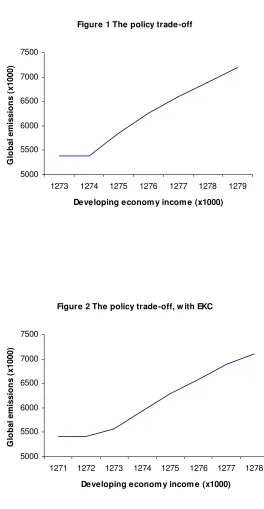
A further key question for those interested in trade and the environment is whether it is possible to increase incomes in developing countries while ensuring no increase in global emissions. An important relationship can be identified as an efficiency frontier that shows combinations of

∑

∑

j i

Eij and Y2 for which it would be impossible to

reduce the former without also reducing the latter by way of changes in e and t. This trade-off is illustrated, for the range of Y2 which can be affected by e and t, by the

upward sloping curves in Figures 1 and 2, respectively for the EKC-off and EKC-on cases. If the current equilibrium is one in which the pairing of global emissions and developing country income is above and to the left of this trade-off, then it is possible to adjust e and t to secure improvement in either or both of these important policy objectives. An interesting feature of this trade-off is seen by comparing the results in Figures 1 and 2. When the EKC is off, the slope of the trade-off becomes flatter as developing country income increases. When the EKC is on, however, the trade-off initially becomes steeper, then becomes flatter.

4. Conclusion

In any model of this type, much inevitably depends on the assumed values of the parameters. Even the qualitative results of studies of this type may be sensitive to the precise assumptions made. This makes the traditional call for further research especially pertinent.

Dasgupta et al. (2002) have argued convincingly that it is likely to flatten out over time. But it would involve an heroic assumption to suggest that it is already absent.

References

Antweiler, Werner, Copeland, Brian R. and Taylor, M. Scott (2001) Is free trade good for the environment?, American Economic Review, 91, 877-908.

Armington, Paul S. (1969) A theory of demand for products distinguished by place of production, International Monetary Fund Staff Papers, 16, 159-178.

Cole, Matthew A. and Elliott, Robert J.R. (2003) Do environmental regulations influence trade patterns? Testing old and new trade theories, World Economy, 26, 1163-1186.

Copeland, Brian R. and Taylor, M. Scott (2004) Trade, growth, and the environment, Journal of Economic Literature, 42, 7-71.

Dasgupta, Susmita, Laplante, Benoit, Wang, Hua and Wheeler, David (2002) Confronting the environmental Kuznets curve, Journal of Economic Perspectives, 16(1), 147-168.

Ekins, Paul (2003) Trade and the environment, in the Internet Encyclopaedia of Ecological Economics, available at http://66.102.1.104/scholar?hl=en&lr=&q= cache:R6aAAC-z3gYJ:www.ecologicaleconomics.org/publica/encyc_entries/ TradeEnv.pdf+

Grossman, Gene M. and Krueger, Alan B. (1993) Environmental impacts of the North American Free Trade Agreement, in P. Garber (ed.) The US-Mexico Free Trade Agreement, Cambridge: MIT Press.

Kuznets, Simon (1955) Economic growth and income inequality, American Economic Review, 45, 1-28.

Perroni, Carlo and Wigle, Randall M. (1994) International trade and environmental quality: how important are the linkages, Canadian Journal of Economics, 27, 551-567.

Table 1 Parameter values

A11 4 A12 1 A21 4 A22 1

α11 0.8 α12 0.7 α21 0.9 α22 0.5

φ11 7 φ12 7 φ21 8 φ22 3

ϕ11 3 ϕ12 1 ϕ21 5 ϕ22 2

ξ11 0.02 ξ12 0.01 ξ21 0.01 ξ22 0.01

κ11 0.05 κ12 0.05 κ21 0.02 κ22 0.05

σ 0.1 L1 0.5 L2 2.5 ρ -1

θ 1 _ζ 1 _γ 0.1 _ω 0.1

Table 2 Results for the EKC-off tariff-on case

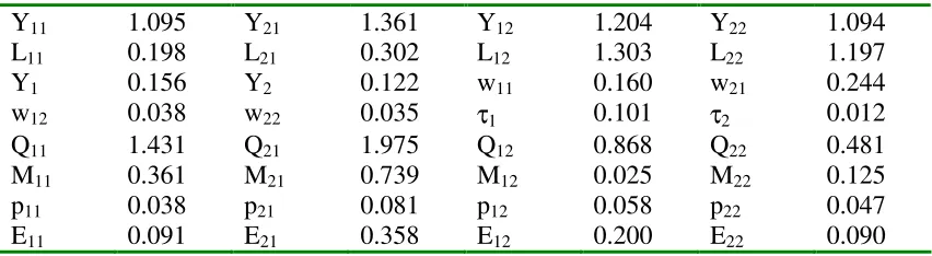
Y11 1.095 Y21 1.361 Y12 1.204 Y22 1.094

L11 0.198 L21 0.302 L12 1.303 L22 1.197

Y1 0.156 Y2 0.122 w11 0.160 w21 0.244

w12 0.038 w22 0.035 τ1 0.101 τ2 0.012

Q11 1.431 Q21 1.975 Q12 0.868 Q22 0.481

M11 0.361 M21 0.739 M12 0.025 M22 0.125

p11 0.038 p21 0.081 p12 0.058 p22 0.047

Figure 1 The policy trade-off 5000 5500 6000 6500 7000 7500

1273 1274 1275 1276 1277 1278 1279

Developing econom y incom e (x1000)

G lo b a l e m is s io n s ( x 1 0 0 0 )

Figure 2 The policy trade-off, w ith EKC

5000 5500 6000 6500 7000 7500

1271 1272 1273 1274 1275 1276 1277 1278

Developing econom y incom e (x1000)