The response of box type structures to vibration

The response of box-type structures to vibration.

HENG, Raymond Bonn Whee.

Available from Sheffield Hallam University Research Archive (SHURA) at:

http://shura.shu.ac.uk/19784/

This document is the author deposited version. You are advised to consult the publisher's version if you wish to cite from it.

Published version

HENG, Raymond Bonn Whee. (1976). The response of box-type structures to vibration. Doctoral, Sheffield Hallam University (United Kingdom)..

Copyright and re-use policy

See http://shura.shu.ac.uk/information.html

THE RESPONSE-OF BOX-TYPE STRUCTURES TO VIBRATION

by

Raymond Boon Whee Heng B.Eng.(Hons.)*

A dissertation submitted to the Council of National Academic Awards for the award of the degree of Doctor of Philosophy

Sheffield Polytechnic

Department of Mechanical and Production Engineering

* at present

University of Sheffield

Department of Mechanical Engineering

ProQuest Number: 10697086

All rights reserved INFORMATION TO ALL USERS

The quality of this reproduction is dependent upon the quality of the copy submitted. In the unlikely event that the author did not send a com plete manuscript and there are missing pages, these will be noted. Also, if material had to be removed,

a note will indicate the deletion.

uest

ProQuest 10697086

Published by ProQuest LLC(2017). Copyright of the Dissertation is held by the Author.

All rights reserved.

This work is protected against unauthorized copying under Title 17, United States C ode Microform Edition © ProQuest LLC.

ProQuest LLC.

789 East Eisenhower Parkway P.O. Box 1346

2^ s

" 7

"o'/?

THE RESPONSE-OF BOX-TYPE STRUCTURES TO VIBRATION

by

Raymond Boon Whee Heng B.Eng,(Hons.)*

A dissertation submitted to the Council of National Academic Awards for the award of the degree of Doctor

of Philosophy

Sheffield Polytechnic

Department of Mechanical and Production Engineering

* at present

University of Sheffield

Department of Mechanical Engineering

Acknowledgement

I would like to thank Mr. G.J. McNulty of the Sheffield Polytechnic and Dr. J.L. Wearing of the University of Sheffield for their supervision of this project. Thanks are also due to my friends and colleagues in both

institutions and in particular Mr. 0. Bardsley, Head of Mechanical and Production Engineering Department, Sheffield Polytechnic and Professor D.E. Newland, Uni­ versity of Sheffield, for help and advice rendered me.

The work described in this thesis deals with the vibration study of an open ended folded plate box type structure leading up to the prediction of its response to random excitation. Theoretical and experimental results for the box are presented as one of the main aims of the work is to predict theoreti­ cally the response of the structure to random excitation

and compare these results with experimentally obtained values using various methods available.

The determination of the response of a structure to random excitation depends on the prediction of the response spectral density. To determine the response spectral density of any point on a structure a knowledge of its natural frequencies and mode shapes and modal damping .factors is required. In this work the finite- element method of analysis is used to determine the natural frequencies of vibration and the

corresponding mode shapes of the box structure and computer programs were developed to perform this analysis. During the project, beam and plate structures have also been

investigated to assess the accuracy of the technique and some results for these are included in chapter 7. The natural frequencies and mode shapes obtained are^compared with experimental results as well as with those obtained using other theoretical analyses. *For the beam the exact method was used and for the plate, the energy method using

Y/arburton's formulae. Computer programs were also developed to calculate the structural receptance from the natural

frequencies and mode shapes calculated using the finite

element technique and damping factors obtained experimentally. From this . the response spectral density of the structure to a known excitation spectrum was obtained.

the development of a non-contacting combined exciter oickup probe, are described and discussed. The response to random excitation is obtained experimentally using a pseudo-random binary sequence signal generator and a time domain analyser, giving the cross-correlation function from which the cross spectral density is calculated in a Fourier transform. A Fast Fourier Transform computer program was developed during

the work to perform this. The response spectral density is then obtained from a knowledge of the excitation spectral density.

Finally the values of the response spectral density obtained 8re compared with those obtained using the results of the finite element analysis and using the results of the sine sweep test and narrow band frequency analysis. The technique 7 used in this work has proved satisfactory and the experimental

apparatus and computer programs developed, suitable for the investigation.

CONTENTS

Abstract

%

Contents Page

List of Figures . *

List of Tables

List of Plates

Chapter 1 Introduction 1

Chapter 2 The Finite Element Method 8

Summary 8

2.1 Introduction 9

2.2 The element stiffness matrices 10

2.2.1 The bending stiffness matrix 11

2.2.2 The membrane stiffness matrix 15

2.3 The element mass matrices 17

2.3*1 The mass matrix in bending 18

2.3.2. The mass matrix in stretching 18

2.4 The combined bend and stretch element :

matrices 18

‘2.5 Assembly into the complete structure 19

2.6 The rotational matrix 22

2.7 Method of assembly 27

2.8 Boundary conditions 27

Contents Page

Chapter 3 Random Theory ^34

Summarj'- - , 34

3.1 Introduction 35

3.2 Basic random theory 37

3.2.1 Statistical approach 37

3.2.2 The correlation functions 40

3.2.3 Power spectral densities 41

3.2.4 Fourier analysis of random signals 42

3.3 Response of structures to random excitation 43

3.4 Experimental techniques 46

3.5 The Correlation technique 49

3.6 The Fourier Transform 51

3.7 The pseudo-random binary sequence 56

Chapter 4 The Apparatus • 64

Summary 64

4.1 Introduction 65

4.2 The vibration test bed 67

4*3 The non-contacting displacement transducer 69

4.4 Development of the non-contacting exciter 70

Contents Page

Chapter 5 Experimental Technique. - 80

♦

Summary 80

5*1 Introduction 81

5*2 The excitation signal 87 *

5*3 ’Experimental technique 91

5*3.1 Determination of natural frequencies &

mode shapes 93

5*3*2 Determination of receptance 97

5*3*3 Determination of damping factors 99

5*3*4 Determination of response to random

excitation 102

5*4 The Past Fourier Transform program 105

Chapter 6 The.Computer Application 108

Summary 108

6.1 Response prediction 108

6.2 The finite element computer program package 112

Chapter 7 Results 128

Summary * 128

7*1 Natural frequencies & mode shapes 128

7*2 Response calculations 143

Contents Page

Plates 170

References ■ ■ * 186

Appendices 1 The stiffness and mass matrices

2 The solution algorithms

3 Finite element suite of computer

programs

4 The fast Fourier transform computer

program

5 The experimental apparatus

6 The Wayne-Kerr probe calibration

List of Figures

Figure . Title Page

2.1 . Element configuration (bending) 12

2.2 Element configuration (stretch) 16

2.3 Element node numbering sequence 20

2.4 Element node renumbered 20

2.5 Degree of freedom notation for the element 21

2.6 Coordinate transformation ₂₃

2.7 Plate orientations 25

2.8 Plate in global x'y* plane 26

2.9 Plate in global y'z' plane 26

2.10 Plate in global z ’x' plane 26

2.11 Assembly procedure 28

2.12 Node numbers of the open ended box structure

analysed l 29

3.1 An ensemble of random signals. 38

3.2 A typical Normal probability distribution 39

3.3 Transient testing signals 48

3.4 A pseudo-random binary sequence signal 58 3.5 Autocorrelation function of a PRBS signal ₅₉

3.6 Power snectrum of a PRBS signal 6.0

3.7 PRBS occurance distribution 62

3.8 Probability distribution of a multi-level sequence 62 4.1 A cut away view of the combined probe 73 4.2 Calibration of vibration pickup transducer - 74 4.3 Frequency response of vibration measurement

transducer 75

4.4 Force output of non-contacting exciter 77 4.5 Effect of air-gap on excitation output 78 4.6 Frequency response of non-contacting exciter 79

5.i Schematic plan of the method * 82

5.2 The vibration pickup displacement-volts factor 84 5.3 The non-contacting exciter force-volts factor 86

5.4 Filter characteristics ₈₉

5.5 The open-ended box structure used 92

5.6 Block diagram of instrumentation for discrete

excitation of box structure ₉₄

5.7 A typical grid for determining mode shane of

Figure Title Page ,

5.8 The grid used, for determining response spectral :

density of the box 98

5.9 Determination of damping factors using half power

points on the response curve 100

5.10 Block diagram of instrumentation for random

excitation of structures 103

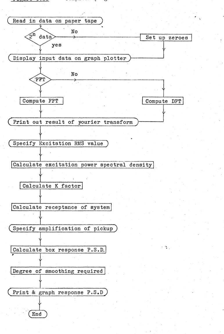
5.11 Computer program MOJFTM flowchart 106

6.1 The twenty-four element idealisation of the box

structure 110

6.2 Computer program M0JFTM1 flowchart 114

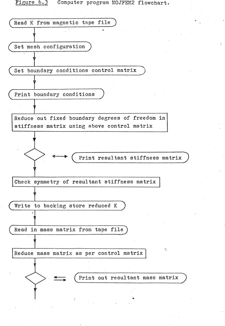
6.3 Computer program M0JFTM2 flowchart 116

6.4 Computer program M0JFTM3 flowchart 118

6.5 Computer program M0JFTM4 flowchart 119

6.6 Computer program MOJFTMD flowchart 120

6.7 Computer program MOJFTM5 flowchart 122

6.8 Computer program M0JFTM6 flowchart 123

6.9 Computer program M0JFTM7 flowchart 124

7.1 1st and 2nd mode shapes of the box 132

7.2 3th and 4th mode shapes- of the box 133

7 .3 5th and 6th mode shapes of the box 134

7.4 7th and 8th mode shapes of the box 135

7*5 9th and 10th mode shapes of the box 136

7 .6 11th and 12th mode shapes of the box 137

7 .7 13th and 14th mode shapes of the box 138

7 .8 15th and 16th mode shapes of the box 139

7*9 17th and 18th mode shapes of the box 140

7.1 0 19th and 20th mode shapes of the box 141

7.11 21st mode shape of the box 142

7*12 The excitation power spectral density used 144

7.13 Showing the points for which response measurements

are presented. ’ 145

7.14 A typical graph plot of the cross correlation /

impulse response function 147

7.15 A typical line printer display of the correlation

function 148

7.16 Box response to random excitation from the

512 point correlation function (non smoothed) 149

7.17 The 5^12 point response PSD curve using a three

Figure Title Page

7.18 The 512 point response PSD curve using a five

point smoothing ~ " 151

7.19 A graph of a nonsmoothed 102^ point response

power spectral density computed 152

7.20 The 1024 poinfr response PSD curve using a

three point smoothing 153

7-21 The 102U point response PSD curve using a five

point smoothing 1

5b

2

7*22 A plot of the typical box receptance calculated

using finite element results 155

7-23 A typical response power spectral density

calculated using the finite element results 156

7.21+ Response power spectral density - Position A 157

7.25 Response power spectral density - Position B 158

7.26 Response power spectral density - Position C 159

7.27 Response power spectral density - Position D 160

7.28 Response power spectral density - Position E 161

7.29 Response power spectral density - Position F 162

List of Tables

Tables

1

2

JPage

Natural frequencies & mode shapes of a beam with fully fixed and simply supported

ends 129

Natural frequencies & mode shapes of a

plate fully fixed all round 130

■u j l^ u u x r j^cl

Plate Title . Page

1 The original vibration table _{• *} 171

2 The redesigned vibration table 172

3 The linear fine adjustment mechanism 173

U The skew fine adjustment mechanism 174

5 The plate with fully fixed edges 175

6 A fixed corner of the box structure 176

7 Close up view of the calibration of the

•capacitance displacement transducer 177

8 Instrumentation for calibration of the

displacement transducer 173

9 Calibration of noncontacting exciter using

a simple beam experiment 179

10 The housing for the piezoelectric force

transducer used for the calibration of the exciter 180

11 Some of the electromagnetic noncontacting

exciters developed 181

12 The combined exciter / pickup in position

over the box structure 182

13 Frequency analysis using constant percentage

frequency analyser 183

14 Constant bandwidth frequency analyser 184

15 The PRBS instrumentation used for the automatic generation of the cross correlation function on

Chapter 1._____ Introduction

The trend in recent engineering development is towards the use of light folded-plate boxtype structures as the basic unit of construction in many fields. In buildings and bri­

dges, box girders figure predominantly and in the transport industry, motor cars, buses and trucks have always been

basically light folded plate box type structures. This has stimulated interest in the determination of the response to vibration stimuli of these structures, hereafter referred to in this thesis simply as b o x - s t r u c t u r e s T h e resulting

reduction in the built-in safety factors as well as in the damping because of the use of these lighter structural mem­ bers can lead to the build up of serious vibration response levels.

Ignorance of the vibration characteristics of such struc­ tures is known to account for premature wear and fatigue failings [lj. The more spectacular catastrophes include the breaking up of the Liberty ships and the bridge disaster at Tacooma, in the U.S.A. where,in the latter case,random wind loading had excited one of the natural vibration modes of the bridge.

In the field of transportation, broad band vibrations set up in the vehicle have been shown to affect not only the life expectancy of the vehicle but also to have undesirable

effects on the commuter. Once again the excitation here is known to be of a random nature. It is therefore important to study the vibration response of box structures and in

particular the response of box structures to random excitat­ ion.

This work is an investigation into the vibration characteris- ics of box structures and ultimately to predict the response of box structures to random excitation. Robson [2] and

(2)

random input at p depends on the determination of the

receptance (Bishop and Johnson [4j ) of the structure at the point under consideration- Hobson has shown that in this case the output spectral density Sd(f) of the point under consideration is related to the input spectral density Sp(f) of the exciting force by the expression:

Sd(f) = |«.dp(if)|2 Sp(f)

(

1

.

1

)

v/here ^ p ( f ) is the receptance of the system from:

(*dp(if) = £ y V Xr “ 1YJ

(1.2)

w r U q)wr (xD)

4 V ’

Mr =./ w 2 (x)mdx ,

f2 - f2

fr

Yr = - f2)2 +

v/r (Xp) and wr (Xq) are deflections of the structure at input and output points p and q respectively when the structure is vibrating in the rth normal mode, fr is the rth natural frequency, f is the forcing frequency and ^ is the damping loss coefficient for the rth mode•

It is therefore possible to calculate the receptance of

any structure given the knowledge of its natural frequencies and mode shapes as well as damping

factors-Any attempt at response work inevitably requires a knowledge of the damping characteristics of the structure. As the mechanism of damping in structures is not yet completely known this work follows a commonly accepted theory for light

structures, that of hysteretic damping (see Crandal [5])*

Experimentally derived values of the loss factors have been used as far as possible for the folded plate box configurat­ ion but where this was not possible, extrapolations were used based on results obtained on plate damping measurements or unimodal damping assumptions were made.

In using equation (1.2) the natural frequencies ,of free vibration and its corresponding mode shapes of the box

structure must also be known. These are obtained by solution of the equation of motion of the structure. Vibration

analysis of structures can be divided into 'exact* methods and approximate methods.

The exact method solves the exact equation of motion usually using an iterative method. This however is only suitable for beams and plates with simple boundary conditions and becomes far too complicated for complex structures. It has not

however prevented a recent attempt by Abrahamson [6] in using the exact method in an analysis of the natural frequencies and normal modes of a four plate box structure. This exact method is well documented in standard dynamics textbooks and will not be gone into here.

Of the approximate methods available the most widely used is the Rayleigh also known as the Energy method used mainly for determination of the lower frequencies of vibration. Here a shape, for example the static deflection curve, is assumed for the true deflected curve. Using this, the maximum

potential and kinetic energies are calculated and equated. If the exact shape of the deflected structure happens to be chosen the calculated frequency corresponding to that shape will also be exactly correct but if not a close upper bound approximation will be obtained [4-1. This method is also limited to the analysis of the simpler structures.

the Rayleigh method with a series of the various characteris­ tic beam functions. This work was extended by others includ­ ing Young [8] in 1950. Both the Rayleigh and the Rayleigh- Ritz methods are well documented in standard vibration text­ books e.g. Timoshenko [9.j and Bishop & Johnson [4]. Probably one of the best known works in plate vibrations was done by Warburton [10] in which he presented a paper giving approxi­ mate formulae for all the twenty one different boundary

conditions possible with plates using the Rayleigh method of solution. Recent work on the same subject was done by Leissa

[ll] who also investivated the effect of changing the values of Poission’s ratio and investigated the accuracy of Warburt- ons formulae.

A theoretical solution to the vibration of box-type structures using a sine series was presented by Dickinson and Warburton

[l2j. The analysis is however limited to the case in which deflections at the corners of the structure are assumed to be zero. The use of the Rayleigh and Raleigh-Ritz methods is in general not suitable for box structures because of difficulty in satisfying continuity of slope and bending moments at the common edges. The transfer matrix method (see Uhrig [l3]) is also not suitable for the box structure because of the

geometric difficulties encountered. The Bolotin edge effect method (Dickinson and Warburton [14]) although able to

satisfy these continuity conditions does not solve for all the modes of vibration of box structures particularly at the higher modes when modal patterns are not easily represented by lines parallel to the edges.

Of the remaining approximate methods available the advent of the high speed large capacity computer has seen the emergence of the finite difference and finite element methods of

analysis. The former (Heng [15]) was possibly until recently the more popular because of its smaller computer storage

It also appears to be the most suitable method available for the analysis of the box structure and is therefore the method chosen for this work.

One of the earliest references using this method was reported in a paper by Turner et.al. [17] in 1956. Melosh [18] sub­ sequently applied it to the analysis of thin plates in bend­ ing. This was followed by Zienkiewicz and Cheung [19] in which they noticed possible application of the method to

include vibration and thermal problems. Dawe [20] presents a solution to plate vibration problems and including non-

dimensionalised stiffness and mass matrices using rectang- * ular elements.

The rapid increase in the use of matrix methods in structural mechanics led to one of tne first major conferences on the subject 121j being held in 1965 at which the finite element method featured predominantly. Since then several textbooks on the method have been published (Przemeiniecki [22] and Zienkiewicz i_23]).

Rockey and Evans [24j applied the method to the static

analysis of box structures. In dynamic analysis, Handa [25] deals with in-plane vibrations of box structures and Ali, Hedge & Mills [26] approximates the vibrations of an idealis­ ed motor car chassis using beam elements only. This project will therefore extend the work to consider the finite element analysis of both in plane and transverse vibration of box structures and to use the results for the determination of the response power spectral density to random excitation. The full potential of the finite element method of analysis is still being constantly increased with new literature on the work being published at the moment in many research establishments.

It is therefore one of the aims of the work undertaken in this project to produce such a computer program package to solve for the natural frequencies and mode shapes of the box structure. These results are then used in the calculation of the receptance of the box structure from equation (1.2).

The receptance is used in the prediction of the response power spectral density to any known input from equation (1.1) and its calculation incorporated in the finite element package developed.

Little work, analytical or experimental, appears in the literature on the vibration study of box structures. As a result an extensive experimental as well as analytical program is pursued to obtains

(a) natural frequencies and mode shapes,with which the accuracy of the finite element prediction of the natural frequencies and mode shapes of the box structure can be assessed, and

(b) the experimental response power spectral density? with which the predicted response power spectral density can be compared.

Although it is not expected that experimentally obtained and analytically predicted results correspond exactly, it is hoped that some degree of collaboration will be achieved.

The experimental work entailed the design and development of suitable experimental apparatus from which the necessary

obtaining the delayed signal for correlation and in the operations involving multiplication and integration. More­ over the perfect repeatibility otherwise unobtainable with pure random signals is here possible making it suitable for work of this kind.

A Fourier Transform is necessary to evaluate the frequency response function of the structure from its impulse response. The calculation is found to require very long computational ' times using the usual method of evaluating the terms. A new technique using the Fast Fourier Transform algorithm (Cooley and Tukey [29], Bingham et.al. [30j , Cochran et.al. [31J) is found to reduce this time considerably and forms an important part of the correlation technique used in this work. The

theory behind this method of calculating the Fourier transform of a series will be looked into in more detail in the

appropriate chapter.

Both the experimental as well as the analytical programme for the box structure has been successfully completed. The

necessary apparatus has been developed and the natural frequencies and mode shape of the box structure have been obtained. The response power spectral density of the box structure subjected to random excitation has been obtained experimentally. A finite element computer program package has been developed giving the natural frequencies, and mode shapes of the box structure. A further computer program has also been developed to predict the response power spectral density of the box structure subjected to random excitation. Agreement between the experimental and predicted results is found to be

Chapter 2 The finite element method

Summary

The Finite Element method is used to predict theoretically the mode shapes and frequencies of free vibration of a folded

2.1 Introduction

The finite element method is one of the most suitable methods for the analysis of complex- structures. In the analysis, whether static or dynamic, the original structure is replaced by an assemblage of small but finite elements which inter­ connect with one another only at a finite number of points known as node points. These are usually found at the corners of the element but are also commonly chosen to be along the sides of the element. At each node a number of degrees of freedom are represented usually the deflections and slopes or their derivatives. The theory then is to assume that the dis­ placements in any part of the element will be defined in terms of these nodal degrees of freedom via a displacement poly­ nomial of the form

w = {P} [C] (2.1)

where {p} is a matrix of the coordinates x,y and z, [C^ is a vector matrix of constants^

and the polynomial w(x,y,z) is chosen to satisfy the following conditions:

(a) The number of independent terms must equal the number of degrees of freedom in the element

(b) For convergence to the correct solution it must be complete up to order n where n is the order of the highest derivative appearing in the strain energy integral appropriate to the type of element under

consideration. ‘

From this displacement polynomial an elemental ’stiffness1 matrix [kl is obtained via strain energy considerations

relating the elemental nodal forces and displacements in the form

{F}e = [k] [d}e (2.2)

In a static analysis the nodal forces {F}0 are due to the applied forces and in a dynamic analysis they represent

inertia forces acting on the element. The characteristics of the complete but considerably simplified structure is then represented on the computer by the equation

. { ? } = D O f a ] (

2

3

where [Kj is the stiffness matrix for the complete structure, made up of all the elemental stiffness matrices [k] . This then relates the applied forces { F } and the nodal displace­ ments [d}of the complete structure and at the same time

satisfies the relevant boundary conditions applied.

2.2 The element stiffness matrices

In folded plate structures the plates are subjected to both bending and stretching effects. This is conveniently

considered separately as the plate element purely in bending and then in stretching only. The former has three degrees of

freedom, w, 0 , 0 at each node and the latter, u and v only._{x y}

2.2.1 The bending stiffness matrix

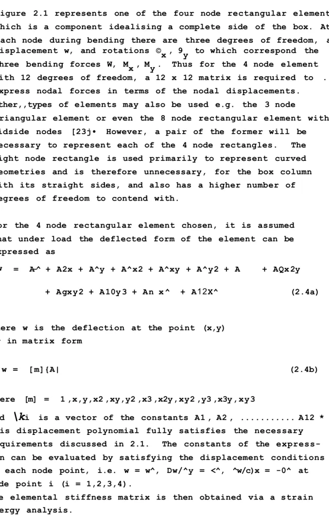
Figure 2.1 represents one of the four node rectangular elements which is a component idealising a complete side of the box. At each node during bending there are three degrees of freedom, a

displacement w, and rotations © , 9 to which correspond the_{x y}

three bending forces W, M , M . Thus for the 4 node element_{x y}

with 12 degrees of freedom, a 12 x 12 matrix is required to . express nodal forces in terms of the nodal displacements.

Other,,types of elements may also be used e.g. the 3 node

triangular element or even the 8 node rectangular element with midside nodes [23j• However, a pair of the former will be necessary to represent each of the 4 node rectangles. The eight node rectangle is used primarily to represent curved geometries and is therefore unnecessary, for the box column with its straight sides, and also has a higher number of degrees of freedom to contend with.

For the 4 node rectangular element chosen, it is assumed that under load the deflected form of the element can be expressed as

w = A-^ + A2x + A^y + A^x2 + A^xy + A^y2 + A + AQx2y

+ Agxy2 + A10y3 + An x ^ + A12X^ (2.4a)

where w is the deflection at the point (x,y) or in matrix form

w = [ m]{A| (2.4b)

where [m] = 1 ,x,y,x2 ,xy,y2 ,x3,x2y,xy2 ,y3 ,x3y,xy3

and

\k

This displacement polynomial fully satisfies the necessary requirements discussed in 2.1. The constants of the express­ ion can be evaluated by satisfying the displacement conditions at each node point, i.e. w = w^, Dw/^y = <^, ^w/c)x = -0^ at node point i (i = 1,2,3,4).

I'D

§\*H os

00

“S

\

.S'* 'S

<1

c

•O Bo <r*

*S-»

_s

(

13

)

Now the bending strain energy U of an isotropic plate of uniform flexural rigidity, D, is given by

ifyC^crdV

O = I

T b/ a [ ( % ) 2+ (^f)2+ 2(^f)p(|%) + 2(1-V)(i?a ) W

‘Vy*0*yx=0L ^x^

oy

^ ^y

dxBy

ic}T [ % ] lc} dxdy D

’y=0Jx=0

and [% ] =

B2w B2w

ro

T P > |CM>

1

ro

*

BxBy

'

V 0

r>

0

(2.5)

(

2

.

6

)

The curvatures can easily be obtained by differentiating equation (2.4a):

d2w 1

{C}

4 ?

d2w dy d2w LdxdyJ

i.e. {Cl = [e ] U }

where [ EJ =

2A^ +

6A

j

X

= 2A^ + 2A^x + 6A1Qy + 6A12xy

A^ + 2Aq x + 2Agy + 3A11x2 + 3A12y2

(2.7)

0 0

0

0

0 0 0 0 0

2 0 0 6x 2y 0 0 6xy 0

0 0 2 0 0 2x 6y 0 6xy

0 1 0 0 2x 2y 0 3x2 3y2

(

2

.

8

)

In order to find the matrix of constants [a} we return to

•where the subscripts refer to the nodal members. In matrix notation

W =

so that = [if^J^d]

Substitution of equations and noting that only [E] strain energy

U = |{d l T (J y = o / x=0 [EJT M [ E ] dx dy) (d j

or U = ^{d]T [K]{d] (2.11)

Applying the theorem of virtual work = F. gives

(2.9b)

(

2

.

10

)

{

f

}

where {F} is the column matrix of nodal forces

i.e. {f} = {W1S Mf*, M01 , W2 » M94 }

[k] is thus the required stiffness matrix and from (2.11)

[K] = [3_1]T ( j , y x!0 [sf[X][E] <3x dy)[B_1] (2.12) where the component matrices [%], |”El and [B- ] are given in

(2.6), (2.8) and the inversion of (2.9a) respectively.

In order to retain the element dimension parameters a and b, the matrix manipulation are carried out by hand giving the matrix

[

kj

2.2.2 The Membranecstiffness matrix

Figure 2.2 represents the configuration and notation used for the 4 node rectangular element in stretching. The dis­ placements in the x and the y directions, u and v, are in­ dependant of each other and so can be considered separately and the analysis is identical in both cases. The displacement polynomial chosen for the displacements in the x direction is

u = AjjX + A^xy + A^y + A^

and that in the y direction is

v = B^x + B^xy + B^y + B^

The assumption for a plane stress distribution is made where

ct^_{Zr Z»} = < w

_{tjJL Li}

By following the same steps as illustrated previously for bending, equations (2.5) to(2.12), the stiffness matrix for the element in stretching is obtained (Appendix la).

2•3 The element mass matrices

In dynamic analysis the nodal forces are induced by inertia loading of the displaced structure. The inertia loading dis­ tributed over an element during vibration is here replaced by a system of equivalent nodal forces by means of the formation of a 'mass* matrix. The criterion adopted for such replace­ ment is that the work done by the equivalent nodal inertia

forces U is equal to that done by the actual inertia forces,

of the element Ua . The former is given by the equivalent

nodal forces j i-n moving through virtual nodal displace­

ments *

i.e.

_{Ue =}

{Vm)-{4v}

(2.13)

The latter is given by the actual distributed inertia loading, [f], in moving through a virtual deflection j wv j

i-e - ua = {f H wv} ' (2.14)

where from (2.4) and (2.10) (wv j = [m ][® "*i{dv ) (2.15)

The inertia force per unit area when the plate is vibrating sinusoidally with circular frequency p is

{ f =y°p2 [m J[B 1 ]{d | (2.16)

where

yD

Thus, equating the work done in bothucases, from equations (2.13) and (2.14)

{dv)T {Pm} = Jy=0

fx=0

which from equations (2.15) and (2.16)

W

M

'

W

S

U

dx ay) f

B_1H

d 1

If each virtual nodal displacement is given the value unity in turn while the remaining displacements are held zero, equation (2.17) becomes

[Pmj =y3 P^[B_3] T (jy=o/x=0 [m]T H dx d^ [B_1]{d }

where [m ] = [ B _1J T (/y^0 /x®0 [mjT [in ] dx dy) [g_1] (2.19)

is the required mass matrix of the element as {F | is the

column matrix of nodal forces representing the inertia loading

on the element/ Once a ain this is derived separately for the

element in bending and in stretching.

2.3.1 Bending mass matrix

From the previous section v/e have that the mass matrix of the

element_is given by

[m] = [b_1J T //[m]T [m] dx dy [b- 1 J (2.20)

For the element in bending [m] is given by equation (2.4) and

[g"1 ] by equation (2.9a) so that [ M ] is easily found (Appendix lb).

2.3*2 Stretch mass matrix

Again the element mass mass matrix considering the stretching case is given by equation (2.20) above. In this case the mass matrix can be divided into two separate submatrices, one for

each direction as they are mutually independant of each other (Appendix lb).

2.4 The combined element stretching and bending matrices

V/e now have the four bending and stretching rectangular plate element stiffness and inertia matrices, [Kg], [Kg], [m^] and

Mg] of the element. These are combined to form the combined bending and stretching stiffness and mass matrices [k ] and [m ]

of the element. These are full 24 x 24 matrices with the

complete set of six rotational and linear displacements u,v,w, 9 ,Q .9 at each of the fou_{x ’ y 5 z} r/nodes. The matrices available

idealised structure more flexible than the actual but has been successfully used (Rockey and Evans [24] , and Clough and Johnson [32]) •

The notation (fig. 2.3) used previously was chosen quite

arbitrarily and was sufficiently suitable for the purposes of determining the stiffness and inertia..matrices of the element. However, it was found that for ease in analysing lare and

complex structures, a more suitable system of numbering for the element had to be followed so that programming for the computer is simpler. The following system (fig. 2.4) was chosen. This gives a smooth flow in the numbering system, considering first the x axis and then the y axis. In the program this is accomplished by first interchanging rows and columns 2 and 4 in the stiffness and inertia matrices and then doing the same for rows and columns 3 and 4. This

procedure is carried out in subroutine REORDER (Appendix 3)*

The complete nodal and degree of freedom notation for an element lying in the xy plane is given in figure 2.5 where, considering node 1,

degree of freedom:

1 = u = displacement in x direction 2 = v = displacement in y direction 3 ~ w = displacement in z direction

4 = 0 =

_A.

2.5 Assembly into the complete structure

The basic element obtained by the previous analysis is a four

node plate element which has combined bending and stretching capabilities.

If we inspect the stiffness matrices obtained we see that a column of either matrix is in fact a list of the forces acting at each node when the displacement corresponding to that

*

I

J

I

1

1

i

kj *

<V

•Cr

8 §

is

V)

■

r

c -K»

/

/

©

0

freedom given the value zero. Thus if two or more elements have a common node point then the total force acting at that node point is obtained by addition of forces. The assembly into the complete structure is then accomplished by the

mering of all the element matrices into that of the complete

structure by a simple point by point addition. The degree of

freedom notation as illustrated in figure 2.5 has been chosen to facilitate easy assembly into the complete structure.

This mering of the basic element matrices into that of the

complete, structure also requires the following

a) rotation of the element into the correct plane before assembly.

b) a systematic assembly of the various elements into the complete structure.

c) a systematic numbering sequence of the nodes of the complete structure to facilitate easy refinement of mesh size.

d) incorporation of the boundary conditions of the complete structure.

2.6 The rotational matrix

So far the stiffness and mass matrices have been found for a plate element in its local coordinate system (i.e. the stiff­ ness and mass matrices have been calculated for the element lying in the xy plane). As an element can also lie in the xz

or yz planes or in any inclined plane, its inclination to the

global axis of the whole structure has to be taken into consideration before it can be assembled into its proper place in the actual structure (see for example Gere and Weaver [33]) ' •

To illustrate the procedure, consider a rod of length L lying on the x axis in the local coordinate system as shown in fig. 2.6. Any point of the rod has components of deflection u,v, and w relative to the local axes x,y and z. It also has

by the expression

tt* =

k)

w*

(

.

)

Prom fig. 2.6,

l(u) = u'cos^u + v'cos v'u + w*cos w*u

where u ’u etc., refer to the angle turned through from the u f axis to the u axis.

Similarly,

l(v) = u*cos u'v +• v'cos v'v + w'cos w fv

l(w) = u'cos u'w + v'cos v'w + v/'cos w'w (2.22)

For the purposes of this investigation the directional cosines invloved are either 1, 0, or -1 since the sides of the box

structure investigated are all at right angles to one another

(fig. 2.7).

i) Consider the case of a plate lying in the x'y' plane fig. 2,8). The matrix is simply:

~ 1 0 0 ~

0 1 0

0

0

1

ii) For a plate lying in the y'z' plane, (fig. 2.9) it is: 0 1 0

0

0

1

1 0 0

and iii) For a plate in the g'x' plane (fig. 2.10) :

Using these rotation transformation matrices, the stiffness and mass matrices of the plate element in its local coordinate system can be transformed into that of the global coordinate system using the equations

1 0 0

0

0

1

0

- 1 0

Co e ,Q

_s

$

c 0

1

and (2.24)

r where

[ R ] =

^21 ^22 * ^ 2 3 X 31 k 32 ^33

(do)

These transformations are performed using the subroutines R0TATE1, R0TATE2, and ROTATE3 for the xy, yz and zx planes

respectively (Appendix 3).

2.7 Me thod of assembly

The priority of assembly of the plate elements into the

complete box structure is as follows. The plate elements are first assembled together to form a complete side of the box. The sides in the xy plane are completed first, beginning with

that at z - 0. The sides in the yz plane are then built up, starting with that at x = 0 and finally the sides in the zx plane, again beginning with the one in the y = 0 position. The method is illustrated in fig. 2.11 showing the priority in which the sides of the box are built up. This priority in the computer program is indicated by the parameter NA in the

calling sequence. The local axes of the elements of each side are as shown previously in fig. 2.8, 2.9 and 2.10. Fig. •2^12 shows the node numbering of the assembled box structure. The above method of numbering of the nodes does not give a narrow band along the diagonal of the matrix in the stiffness and mass matrices. In a dynamic analysis however, this does not present the same advantage it would using a narrow band solution in static analysis.

2.8 Boundary conditions

cA

I

i

(29)

3

§

§ .

c/

o

o

--OO

Oa

VX>

U

I

!

o

l

>5 '•'Q

is

.rs, §_o X:

£< <N • 0\

•S^ y

corresponding to that particular degree of freedom. This is because the inertia forces produced in such a case is non -<existant since no displacement is allowed at that point. In

this way a fully fixed node at*the boundary.of the structure may have all its degrees of freedom u , v , w, 9 , 9 , 9„_{x y z}

eliminated from the system matrices. Similarly a node along a simply supported boundary along the x axis may have rows and columns corresponding to its w and 9X displacements

removed. Other*degrees of freedom that are also reduced out are those of dummy nodes and the dummy degree of freedom 9_ which had been assigned for ease of assembly. Where there are no contributions to the assembled stiffness and mass matrices the relevant rows and columns (which are all zeros) are removed from these matrices as they would otherwise

become singular. The removal of these rows and columns is achieved using a control matrix in which a list is maintained of all the degrees of freedom of the structure, those to be

removed represented by zeros and those to be retained by ones.

The subroutine BOUNDARY removes all rows and columns

corresponding to the degree of freedom having the value zero, leaving n by n stiffness and mass matrices where n is the

total number of degrees of freedom remaining in the structure.

2.9 The solution algorithm

The structural vibration problem (section 2.3) is now reduced to one of solving the generalized symmetric eigenproblem

[k ] x = X

[

for its eigenvalues and eigenvectors. Prom these are obtained the natural frequencies and mode shapes of the

vibrating box structure. A short summary of the method used is given here and the reader requiring more detailed informat­ ion is referred to the computer subroutine manual used [34J and Wilkinson [35]•

For the generalised symmetric eigenvalue problem where [k] is

than zero, the solution is straightforward. {.Ml is factorised by Choleskyfs method into {.Ml = {^l] where [L] is a

lower triangular matrix. Hence [k]

I

in the form

( [l]- 1 [k ][l]"T)[l]Tx = \[l)Tx (2.26)

which is the standard symmetric problem

[A]y = Xy (2.27)

where [a ] = [l]"1 [k

and . y [t]T x

The eigenvalues of [K]jx\ = X{m]{x} are the same as those of [A] and

if y is an eigenvector of [A] then x, the corresponding eigen­ vector of the original problem, is obtained by back substitut­ ion in the set of linear equations

[L]T x = y (2.28)

Householder’s method is then used to tridiagonalise the matrix

LA]

only be used if [K] is real and symmetric and \M] is positive definite. [K] is checked to be real and symmetric by inspect­ ion and in the computer program. The program also has built

-in facilities to check the eligibility of {.Ml us-ing the

criterion that its determinant is positive since the determin­ ant is equal to the product of its eigenvalues (which must all be greater than zero)•

In some instances due to rounding errors [M] may not be found to be positive definite so that an alternative method has to be used. The procedure commences with the generalised

symetric eigenproblem being manipulated into the standard symetric form

where

[

q

]

and \ « B 1A

_\

* _ *1

The [K] and [M] matrices are both symmetrical but since [Kl is not,so neither is the product []. The problem then

becomes one of solving for the eigenvalues and eigenvectors of equation (2.29) where [B] is an unsymmetric matrix. An

iterative method applied to this [g] matrix then proceeds to

find the lowest natural frequency first directly.

Because the elements of the matrix [] often varies consider­

ably in size, the process of balancing is used. This is the.

name given to the rearrangement performed, necessary to obtain maximum accuracy in the subsequent solution for the eigenvalues and eigenvectors. The object of balancing is to make the norm (the sum of the absolute values of the matrix elements in each row or column) the same order of magnitude in the corresponding rows and columns. Error in the calculat­ ion of the eigenvalues of the problem is reduced since the eigensolution program used produces results with errors found to be proportional to the norm of the matrix.

The solution then follows with similarity transformation on the balanced matrix [a] s o that U ) is transformed into the real upper Hessenber matrix [h] where [h] = [s]“^[a][s.] An

upper Hessenber matrix is one whose elements h ^ are such

that h .. = 0 when i - j >1. The transformation matrix [s] is built up as the product of n-2 stablised elementary transfor­

mation matrices, chosen so that the eigenvalues and eigen­ vectors of [h] can be more readily determined than those of

[a]. The eigenvalues of [h] are the same as those * of [a] and if y is an eigenvector of [h] then [s] y is the corresponding eigenvector of [a]. The transformation process is however considerably simplified because of the balancing already carried out and only part of the matrix is operated upon. There is no simple method for easily calculating selected

eigenvalues of an upper Hessenber matrix and all eigenvalues

time and storae may be made if only at most 25 percent of the

eigenvectors are required. Since more than this is required it is actually more efficient, both in time and storae, to

use back substitution subroutines which calculate all the eigenvectors and then to discard those that are not needed. The QR algorithm[36]is used in the eigensolution subroutine. This is a very stable method but accuracy is dependant on the eigenvalues being well spaced out.

Chapter 3 Random theory

Summary

This chapter describes the basic terms and concepts of

random theory. The significance of the correlation function of the excitation and the response signals for the case of white noise excitation is discussed. The Pseudo random binary sequence signal is a convenient white noise signal suitable for use in obtaining the cross'correlation function easily and giving the system impulse response function. The receptance of the system is obtained by a Fourier transform of the system impulse

response and calculation of the discrete Fourier trans­ form using a new and faster technique is used. It is also shown that the frequency analysis of any response to random excitation is not accurate and an alternative method of determining the response in form of its power

3.1 Introduction

Knowledge of the response of structures to random excitation of any given type of spectrum is important. This chapter

deals'with the background theory relating to random

excitation of a folded plate box type structure which may

represent a car travelling along an uneven, road surface, an

aircraft subjected to high speed air turbulence or buildings

and bridges to wind gusts. A brief description of basic random signal theory is given. The reader requiring a more detailed knowledge of random vibration theory is referred to standard text-books e.g. Robson

[2~]

A truely random process is by definition unpredictable. In order to make possible any analysis at all a statistical type solution of the response of structures to random excitation must be relied upon. Moreover it is difficult experimentally

to generate a true random signal and to be able to reproduce it again when required. The use of a special type of random signal overcomes these difficulties.. This is known as the pseudo

random binary sequence and will be discussed later in this chapter.

The response of structures to random excitation is discussed and the theoretical basis for its experimental as well as analytical derivation is examined. The method used in this

work to determine this response experimentally is based on the

time domain correlation of the input and response signals. For the special case of a flat excitation spectrum the cross

spectral density obtained on performing a Fourier transformation on the cross correlation function also gives the frequency

response function or receptance of the structure.’ The advantage

resulting in the elimination of interference signals greatly en

Robson also shows (eqn. 1.2) that the receptance of a structure can be calculated from a knowledge of its natural frequencies and mode shapes. He provides the theoretical basis for the

prediction of the response spectral density from this receptance as well as the knowledge of the excitation power spectral

density.

The finite element method of analysis described in the previous chapter enables the calculation of natural frequencies and

3.2 Basic Theory

Before going into the realm of random vibration some of the basic theory and concepts of random processes as given in [2] are here reviewed, and basic terms peculiar to random theory are defined.

3.2.1 Statistical approach

\

Because random signals are by definition unpredictable they can only be described in statistical terms. The basic

requirement of such a description is an 'ensemble1 of time series records of the signal (fig 3*1) which may represent force, acceleration, displacement etc.

One common way of describing the signal statistically is by means of its probability density distribution p(x) which is defined so that

Prob [x$x(t )'£x + dt] = p(x)dx (3.1) where the total area under the p(x) curve is equal to one, and indicates that the probability of the signal lying be­ tween extreme limits of the curve is 100

%

occuring random signals have a bell shaped probability density function (fig 3.2) given by

p(x) = 1 exp[---ifpl-] (3.2V

2 ic

where is the mean square value, also called the variance of the signal and m is its mean.

*

«

s

)

1

•

S c e

o

-

o

s.

N)

In practice analysis is simplified by the introduction of the concept of the ‘stationary* random process. This is one in which a probability distribution obtained for a particular record is identical to those obtained for all the other re­ cords and is therefore independant of the time at which the

record is taken. All the statistical characteristics of a stationary random process e.g. its mean, mean square etc. are therefore time invariant. This concept is taken a step further

by the introduction of the erodic process which is defined as

not only being stationary but also has its probability distri­ bution taken across the ensemble identical with that taken along any particular record.

3.2.2 The correlation functions

The correlation of the excitation and response signals of the

structure will be used in later calculations and provides an

important means of signal analysis.

The auto-correlation function Rxx(t,z) is defined as the averae over several records of the product of x(t) and its

delayed version x(t+z) which for a stationary signal is

Rxx(z) = E [x( t)x( t+z)] (3• 3)

where E represents the avera process.

Similarly the cross correlation function Rxy(t,z) of two stationary signals x(t) and y(t) is

Rxy(z) = E[x( t)y( t+z)] *(3.4)

so that in the limit as z — oo ,Rxy(z)->0

This is because there is no correlation between two different signals at that period of delay and this important property