The Economic Reunification of Korea: A Dynamic General Equilibrium Model

Munich Personal RePEc Archive

The Economic Reunification of Korea: A

Dynamic General Equilibrium Model

Bradford, Scott C. and Phillips, Kerk L.

Brigham Young University

February 2008

Online at

https://mpra.ub.uni-muenchen.de/23550/

The Economic Reunification of Korea:

A Dynamic General Equilibrium Model

Scott C. Bradford

Department of Economics

P.O. Box 22363

Brigham Young University

Provo, UT 84602-2363

phone: (801) 422-8358

fax: (801) 422-0194

email: [email protected]

Kerk L. Phillips* Department of Economics

P.O. Box 22363

Brigham Young University

Provo, UT 84602-2363

phone: (801) 422-5928

fax: (801) 422-0194

email: [email protected]

February 2008

Keywords: factor mobility, dynamic general equilibrium, specific-factors, Korea

JEL codes: F15, F22, F42

*

Abstract

This paper constructs a dynamic specific factors model to examine the impact of the

economic reunification of North and South Korea. The model is a compromise between the

highly stylized neoclassical models of trade found in the theoretical trade literature, and the

highly aggregated models used in dynamic macroeconomics. We find that the policies with the

biggest effects on aggregate output are changes in government tax and spending rates,

particularly spending on infrastructure. In contrast, we find that both skilled and unskilled wages

are much more responsive to the particulars of trade policy, particularly openness to intra-Korea

trade and intra-Korea labor mobility. The location of production in a fully integrated Korean

1 Introduction

When World War II ended on August 15, 1945, Japanese forces occupying Korea south of

the 38th parallel were directed to surrender to US forces. Those in the North surrendered to

Soviet forces and Korea was effectively divided. Ideological differences led to the establishment

of two separate governments in 1947 and 1948. In June of 1950 war broke out and the ensuing

stalemate has left Korea divided ever since.

Recent political events have made the prospects for Korean reunification quite dim. Despite

this, Koreans on both sides of the border express strong desires to reunite. There seems little

doubt that given the right political climate reunification will occur.

In the six decades since Korea was divided much has changed. The economic miracle in

South Korea is well documented and widely studied. Following the Japanese model of export

oriented growth, output grew rapidly in the 1970’s and 1980’s and the South still maintains a

relatively high annual average real growth rate. South Korea today enjoys a robust, healthy

economy.

The Japanese occupation left the North with greater industrial capacity, but much of this

was destroyed by the Korean War. During the Cold War, the North nimbly played on

animosities between its two main benefactors, China and the Soviet Union, and made remarkable

progress in standards of living. However, things have changed since the demise of the Soviet

Union. Markets for North Korean manufactures have all but disappeared. While China does

supply some aid, it is nowhere near the levels the Soviet Union used to provide. Famines have

repeatedly swept through the country in recent years due to a combination of poor agricultural

management policies and unfortunate weather conditions.

While the South has continued to grow and now enjoys per capita GDP on par with those of

many developed nations, the North has slowly slid into poverty. South Korea trades heavily with

the rest of the world. North Korea is isolated and its economy bears a remarkable resemblance to

old Korea, which was often called the Hermit Kingdom for its closed borders and reluctance to

deal with outsiders.

If reunification occurs anytime in the near future the huge differences in standards of living

are likely to cause radical adjustments. With 22 million people in the North and another 47

million in the South the problems will be at least as daunting as those that confronted East and

West Germany over a decade ago. Indeed, given the larger difference in standards of living and

This paper focuses on the likely consequences of the reunification of the two Koreas. We are

interested in several questions. There is little doubt that North Korea will benefit from almost

any change in economic policy. We examine the effects of various kinds of reform on the North

Korean economy. These range from internal reforms that encourage the establishment of

markets to complete economic integration with the South. While happenings in the North are of

vital importance to the lives of millions, the questions facing the South are more subtle, and

hence have less obvious answers. Will the South benefit on net from reunification? Who will

gain and who will be harmed? South Korea is already an open economy. How large can the

benefits of preferential trade with an economy as backward as the North be? How much will

South Korean wages and standards of living be lowered due to competition from workers in the

North? We attempt to address these questions using a calibrated dynamic general equilibrium

model of the North and South Korean economies.

Of course, we are not the first researchers to examine the economic consequences of reform

and reunification on the Korean peninsula. For obvious reasons, researchers in Korea have

examined this issue for many years. Shim (1993) is a good example; it focuses on the optimal

timing of various reform and unification policies. Most work in this literature has concentrated

on the politics of reunification, however, and the economics have not kept pace with

developments in macroeconomic and international trade modeling.

Notable exceptions to this generalization are Noland, Robinson & Liu (1999) and Funke &

Strulik (2005). The first paper calibrates a multi-sectoral computable general equilibrium model

(CGE) for North and South Korea for 1990. Funke & Strulik (2005) set up an endogenous

growth model and examine the dynamics of reunification. They consider the role of

interregional transfer payments and government budgets, issues which we ignore in this paper.

The biggest area of difference between our model and these is in the dynamics. Our model is

based on discrete-time dynamic programming tools used widely in dynamic stochastic general

equilibrium (DSGE) macroeconomic models, albeit the simulations we perform are

non-stochastic. Noland, Robinson & Liu (1999) impose calibrated reduced-form dynamic equations,

while Funke & Strulik (2005) calibrate continuous time structural dynamic equations. Our

characterization of technology and its evolution over time also differs. Our model focuses on

implementation of the current best worldwide technology and the role of infrastructure.

Our choice of a modeling framework is not entirely new, though its application to Korean

unification certainly is. Both Eaton (1987) and Roldos (1991) presented early work on dynamic

as optimally acquired financial assets. Using labor as the mobile factor, he focuses on the

conditions under which the dynamic model displays behavioral properties similar to the static

model. Roldos used a model conceptually very similar to ours to examine the effects of various

types of tariffs on the current account. More recent uses include: Kose (2002), which uses a

similar model to find the proportion of business cycle movements in developing economies

attributable to international price fluctuations; and Albert & Meckl (1998), which examines the

role of qualitatively rational expectations in capital accumulation.

Our choice of a model is motivated by the simple and well-understood properties of the

specific factors model along with a desire to build a model that can be calibrated to reasonably

mimic the actual North and South economies.

We model skilled labor as specific factors and capital and unskilled labor as mobile factors.

We also model defense considerations by having a government that invests in military capital

and conscripts workers to provide some chosen level of defense.

Once this model is calibrated we can examine a variety of reforms and types of reunification.

We first derive and calibrate a baseline model in sections 2 and 3. This baseline model assumes

profit maximizing firms and utility maximizing consumers. For this reason it does not

correspond to the current situation in North Korea. We interpret this baseline as the situation

that would prevail if the North were to adopt internal economic market reforms, while remaining

closed to trade and maintaining defense parity with the South. Section 4 examines the impact of

trade liberalization, defense reduction, a free trade arrangement, coordination of common

macroeconomic policies and full integration. It also considers a scenario where these reforms

are phased in over time. Section 5 concludes with a summary of the results and suggestions for

further research.

2 A Dynamic General Equilibrium Model

We build a model with infinitely-lived households that maximize discounted lifetime utility.

They derive utility from consumption of a single non-traded final good, which can also be used

to form capital of various types. This final good is produced using a set of J intermediate goods.

We treat this good as non-traded because we consider the production of final consumption and

capital goods as something that must be done on site. To build a factory, a firm may purchase all

the necessary materials, but it still needs to assemble the parts – it cannot import the factory

completely preassembled. Assuming non-traded capital means that the capital account is always

Intermediate goods are produced using three factors: capital, unskilled labor, and skilled

labor. We choose these three factors based on data from the Global Trade Analysis Project

(GTAP) which reports payments to five different factors. Two of these, natural resources and

land, are not used in the manufacture of all goods and together contribute less than five percent

of national income. We ignore these two and build a model around the remaining three factors.

Skilled labor is assumed to be specific to the industry in which it is used; that is, it cannot be

used to produce any other intermediate good. Both capital and unskilled labor are mobile across

all J sectors. Skilled and unskilled labor are assumed to be fixed by endowment, while capital is

accumulated optimally over time. Capital and both kinds of labor are non-traded. Intermediate

goods can be traded or non-traded and we calibrate the model accordingly once we identify each

of these sectors.

Conceptually, it might seem more natural to think of capital as a specific factor; capital goods

are certainly more specialized for specific tasks than skilled labor is. However, capital is

accumulated and depreciates over time making it a de facto mobile factor. If we were to model

capital as having J different types, each specific to a particular intermediate good, the only

substantive difference between that model and ours would be a non-negativity constraint on

investment for each type of capital. Since skills are generally task specific, skilled labor is more

likely than unskilled labor to be immobile across sectors.

The government engages in two activities, accumulation of infrastructure capital and

provision of national defense. We assume it imposes lump-sum taxes each period to provide

public investment in infrastructure and military capital. It also imposes conscription on unskilled

labor which is used along with military capital to provide a desired level of national defense. We

impose conscription on unskilled labor only as this seems closest to what is actually done. Most

soldiers are conscripted at relatively young ages before they have acquired any special job skills.

In the long-run the economy grows because of exogenous technical progress. Since both

countries are small, the progress comes primarily from overseas and we impose a constant

growth rate for this external process. Domestic productivity levels are assumed to be influenced

by the level of infrastructure, however, and changes in the stock of infrastructure can therefore

have short-run effects on the growth of domestic productivity.

We now proceed to formally setup and solve the model for a single economy.

Households are infinitely-lived and maximize the discounted sum of all lifetime utility. We

write this optimization as a standard dynamic programming problem using the following

Bellman equation: )} ' , ' ( { ) ( Max ) , (

' + Θ

=

Θ U C E V K K

V

K β (2.1)

where C is the household’s consumption, β is the rate of time preference, K is capital stock,

Θ is its information set used to take expectations, and the primes indicate values of variables next period.

Consumption is income from skilled labor (L), unskilled labor (N), and capital, less

depreciation, investment in new capital, and lump-sum taxes (T) as below.

T K K r N f v L w C i i

i + − + + − − −

=

∑

where wi is the wage rate for skilled labor in sector i, v is the wage for unskilled labor, r is the

rental rate for capital, δ is the depreciation rate, and f is the government conscription rate.

We assume a constant elasticity of substitution utility function of the following form:

σ σ − − = 1 1 1 )

(C C

U (2.3)

Hence, the Euler equation associated with this optimization problem is:

)} ' 1 ( ' { δ β σ

σ ₌ − _{+ −} −

r C

E

C (2.5)

Final Goods Producers

The final goods sector is perfectly competitive with free entry and zero profits. Firms

therefore solve the following profit maximization each period:

∏

∑

∑

F F PF a

j j 1 ; Max }

{ (2.6)

where Fj is the amount of good j used in production of the final goods and Pj is its price.

The first-order conditions reduce to the following J conditions:

Y a F

P_{j j} = _j ; ≡

∏

j a j j

F

Y j _(2.7)

Intermediate Goods Producers

Intermediate goods are also competitively produced and the firms solve the following

problem: j j j j c b j c j b j j j N L

Kj j j PK ZN ZL rK w L vN

− −

− =

Π 1− −

,

, ( ) ( )

where Z is an economy-wide level of domestic productivity which is driven by external

productivity and domestic infrastructure.

The first-order conditions reduce to the following 3J conditions:

j j j bPY

rK = ; Y K ZN ZLj b c j

c j b j

j ≡ ∀

− − 1 ) ( )

( (2.9)

j Y cP

vNj = j j ∀ (2.10)

j Y P c b L

wj j =(1− − ) j j ∀ (2.11)

Government

The government imposes taxes to build up the domestic stock of military capital (M) and

infrastructure (I). Gross investment in these two capital stocks is indicated by a preceding Δ. The government’s budget constraint is:

I M

T =Δ +Δ (2.12)

Military capital and infrastructure evolve over time according the following two laws of

motion:

M M

M'=(1−δ) +Δ (2.13)

I I

I'=(1−δ) +Δ (2.14)

The government also conscripts soldiers from the ranks of unskilled labor. It combines these

soldiers with the military capital to produce a level of national defense as shown below:

d d

ZfN M

D= ( )1− (2.15)

Technology

There are many ways that infrastructure may influence technology1. We assume the

economy-wide technology level, Z, evolves over time as a function of the external level of

technology and the domestic level of infrastructure per unskilled worker:

h h

N I z

Z = ( / )1− (2.16)

where z is the world technology level.

This formulation is intended to capture movements in total factor productivity (TFP) that are

unrelated to technology, per se. It explains how, even though the North has access to the same

technology internationally, it has generally lower total factor productivity than the South. Using

1

infrastructure per unskilled worker assumes that infrastructure is primarily rival in nature and

that greater amounts are needed for a larger population. We use unskilled workers rather than

the sum of skilled and unskilled labor for analytical ease in simulations with internationally

mobile factors. As a result, when skilled labor is mobile between the North & South, these

movements will not generate congestion effects, but mobility of unskilled workers will.

External technology grows at a predetermined constant rate of gz each period.

z g

z'=(1+ _z) (2.17)

Combining (2.16) and (2.17) gives a law of motion for Z that depends on last period’s level

and the growth rate of the infrastructure stock.

Z g g

Z'=(1+ _z)h(1+ _I)1−h ; I_I I

g '

1+ ≡ (2.18)

Aggregation and Market-Clearing

The final goods market and the markets for capital and both kinds of labor are closed to

imports, so domestic supply must equal domestic demand. Intermediate goods may be either

closed or open to trade. We adopt notation that allows for all intermediate goods to be traded,

but will impose zero export restrictions in the appropriate industries.

The aggregation and market-clearing conditions are:

capital stock aggregation,

∑

=

j j

K

K (2.19)

unskilled labor market clearing,

∑

= −

j j

N N

f) 1

( (2.20)

skilled labor market clearing,

j L

Lj = j ∀ (2.21)

intermediate goods market clearing,

j X F

Y_j = _j + _j ∀ (2.22)

and final goods aggregation

I M K C K

Y+(1−δ) = + '+Δ +Δ (2.23)

The above sections define a model with growth. Some variables - such as, consumption,

capital stocks and production - grow at the rate gz in the steady state. Others, such as goods

prices, remain constant. In order to solve the household’s dynamic programming problem we

rewrite the system in a stationary form by dividing all growing variables by Z. This yields a

steady state where all values are constant and where the off-steady-state dynamics are

characterized by convergence to these constant values. We solve this altered set of equations,

but then readjust once we are done so that all growing variables have the appropriate growth

component added back in our simulations.

The model as a whole has three endogenous state variables, K, M & I. It also has three

exogenous policy variables which should also be viewed as state variables. These are the

conscription rate, f, and decisions about the accumulation of infrastructure and military capital.

We choose to characterize government policy as the percent of Y that will be allocated as

investment in these two stocks. We define the following i≡ΔI/Y and m≡ΔM /Y and model

the government as setting these exogenously. Hence, the exogenous state variables are f, i & m.

We solve the model first by searching for a set of prices that yield steady state exports and

imports equal to the averages observed in the GTAP dataset. We treat the prices for sectors the

traded intermediate goods as fixed international prices and use these constant relative values for

all simulations. The prices in the non-traded sectors are autarky prices and are part of the

solution for each simulation.

As long as the North and South have no unique trading relations, we can treat each as an

economy in isolation2 and solve a one-economy model for each country. We treat production

capital, K, and infrastructure I, as our endogenous state variables. We also solve for the

non-traded intermediate goods prices as endogenous non-state variables. We impose the stationary

versions of (2.5) and (2.18) along with four restrictions of zero imports for the non-traded sectors,

three restrictions on relative prices for the traded sectors, and one price aggregation constraint

relating intermediate good prices to the price of final output (our numeraire) to give us a system

of ten equations in ten unknowns which describes the steady state.

In the scenarios where there is a free trade arrangement or intra-Korea mobility of labor, we

solve a two-country version of the model. In this case we have capital and infrastructure in both

regions as endogenous state variables and prices as endogenous non-state variables. We impose

the North and South versions of (2.5) and (2.18) as above. For the non-traded sectors we impose

2

the constraint that the sum of exports from both regions must be zero. All other conditions are

the same as the one-country case. This yields a system of 12 equations in 12 unknowns.

In addition to the steady states, we are also interested in transition dynamics. The numerical

techniques for solving these types of dynamic problems are well-known.3 They require the use

of the same system of equations used to find the steady state. We use the method of

undetermined coefficients to solve for a linear approximation to the intertemporal decision rules

for capital and infrastructure about their steady state values. With these rules in hand, we are

able to examine the path of key macroeconomic variables from some initial state to the steady

state that are implied by a variety of policies.

3 Baseline Model Calibration & Simulation

We calibrate our model by choosing a baseline scenario where both the North and South are

open to trade. From this baseline we consider various degrees of economic cooperation and

integration between the North and South. We base much of our calibration on data from South

Korea. Where possible we use the limited data on the North Korean economy. In many cases,

however, we are forced to assume that the North looks similar to the South and calibrate using

data from South Korea.

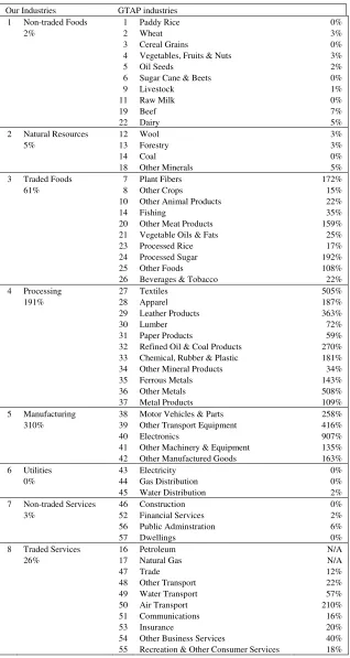
Our first task is to aggregate the 57 industries in the GTAP dataset into a smaller and more

manageable number. We distinguish between foods, processing, manufactured goods, utilities

and other services. We examine the GTAP data for South Korea and discover that foods and

services have a great deal of variation of total trade as a percentage of output across the various

GTAP industries. We divided each of these sectors into traded and non-traded sectors using a

cutoff of 10% of output as the criterion for a traded good. Non-traded foods include grains and

other staples. While North Korea trades very little, these foodstuffs are a large portion of that

trade. Since these foods are non-traded in the South due to trade barriers, we will continue to

treat them as non-traded in the North Korean case, under the assumption that the North will

impose similar agricultural protection. GTAP does not report imports and exports of oil and

natural gas which are not produced in Korea. We assume that our last industry, traded services,

includes imports and exports of oil, natural gas. Table 1 summarizes this information.

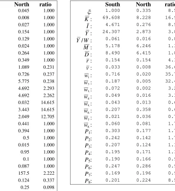
For calibration purposes our time-period is one year and we choose our parameter values

accordingly. We need to set the following parameter values for both countries:

3

z i b c h g

a}, , , , , , ,

{ β δ σ . In addition we need to pick values for labor endowments,{L_i}&N, and

world prices, {P_i}, for traded intermediate goods.

β, the time discount factor is set to .975, implying a subjective discount rate of 2.56%; δ, the depreciation rate is set to .10, and gz, the international trend growth rate of technology is set

to .015. The steady state version of equation (2.5), written below as (3.5), is used to choose the

value of σ, the intertemporal elasticity of substition.

)} 1

( ) 1 (

1=β +gz −σ +r−δ (3.1)

We set the user cost of capital, r −δ , equal to 3% and solve to get σ =.087. All these values apply to both the North and South.

We use data from GTAP (version 5) to find the share of capital and unskilled labor in GDP

for South Korea. These values are b=.4414 and c=.3943.

The values for the ai’s come from aggregating the 57 industries in the GTAP dataset into

eight and finding their output shares as a percent of total output. Again, this is done for South

Korea.

The GTAP data show that total compensation for skilled workers is about 40% of the total

compensation of unskilled workers. Since wages should be higher for skilled workers this is an

upper bound on their number. We assume an unskilled labor force of 300 and a skilled labor

force of 100. To calibrate the distribution of skilled labor over our eight industries we assume a

common real wage and make each labor endowment proportional to total compensation. When

we calibrate North Korea we will choose different values for the Li’s, using this baseline as a

reference.

For 2002 – 2004, the Republic of Korea spent 2.21% of GDP on “social infrastructure and

housing” and “information technology” and another 2.45% on defense. We therefore set

m=.0245 and i=.0221. The population aged 15 or older is 33 million and the non-military labor

force is 22 million. Figures for the military are harder to document, but most sources indicate it

has roughly three-quarters of a million men under arms. Since we have already assumed that

three-fourths of the labor force is unskilled, the conscription rate on unskilled workers is either

2.92% of the population or 4.18% of the labor force. We use the latter value.

For North Korea we keep the same values for b, c, h, gz, β, δ & σ. The total population in

North Korea is around 23 million versus South Korea’s 48 million. We set overall labor to 180;

difficult to pin down. For lack of defensibly better numbers, we assume that the percent of the

total labor force that is skilled is half the value we use for South Korea. That is 12.5%, rather

than 25%. This gives N=157.5 and Li’s that sum to 22.5. The allocation of skilled labor across

industries is calibrated using data on similar industrial classifications from South Korea’s

Ministry of Unification. When this data does not match our 8 industries exactly we impose

ratios similar to those observed in South Korea. The exact distribution of skilled labor is shown

in the first panel of Table 2.

For policy variables we take a military force of one million and divide by 87.5% of the 9.2

million labor force and round to get f=.124. Determining the values of military and

infrastructure parameters is the most problematic of all. The value of m=.25 is chosen to give the

North and the South roughly equal levels of defense in the steady state for our baseline. i is set

to half the value of the South. We note that our simulation is for a case where reforms have been

instituted in North Korea and need not reflect exactly current economic policy.

The values of all the parameters and the steady state values for this baseline model are also

reported in table 2.

We assume that initially neither the South nor the North is in the steady state. This means we

need to choose starting values for five values: capital stocks in both countries, infrastructure in

both countries, and the relative level of technology in the North.4

South Korean growth rates per capita are greater than our steady state value of 1.5% per year,

and have a gradual downward trend. We constrain the initial ratio of private capital to

infrastructure to be equal to the steady state ratio and then choose initial values for the capital

stock and infrastructure so that the initial growth rate in the South is 5% per annum, roughly the

average real growth rate over the last five years.

We need to know the difference between technology in North and South Korea. We use

(2.16) and define the relative technology measure, ξ ≡ZN /ZS to get h

N S

S N

N I

N

I −

⎟⎟ ⎠ ⎞ ⎜⎜

⎝ ⎛ =

1

ξ (3.2)

4

Choosing a value for the initial infrastructure in the North also determines the initial level of

technology. We assume that infrastructure in the North begins 15% below its steady state value.

We assume capital is also 15% below steady state.

These assumptions yield an initial per capita income level in the North that is 16% of the

South’s. The baseline model assumes that North Korea is characterized by agents responding

optimally to market signals. Since this is obviously not the case now, we must interpret this

model as a scenario where the North has already engaged in some kind of market reform. Our

starting values give GDP in the South that is almost fourteen times that in the North. However,

the Ministry of Reunification estimates that South Korea’s GDP was actually 26.8 times that of

North Korea in 2001. This implies that internal reform in the North would result in efficiency

gains that roughly double output.5

We wish to remphasize that the values used in our simulations are very rough approximations.

As a result we have little confidence in the exactness of the numbers from our simulations.

Particularly for the North our numbers can serve only as very rough guides as to the general

direction and magnitude of changes.

Given these starting values we proceed to simulate the model economies.

4 Scenarios

With the model solved, calibrated and simulated for a baseline case, we now proceed to

consider various steps on the road to unification. These steps include changes in international

trade policy and in other economic polices. We consider the steady states of six scenarios in

addition to the baseline. Some scenarios are unlikely. Our baseline where the North institutes

market reforms but does not open to international trade, for example. We present them

nonetheless to isolate the effects of each of the various policy changes.

These are as follows:

• Scenario 2 –Baseline, plus North opens to world trade.

• Scenario 3 – Scenario 2, plus both North and South reduce defense.

• Scenario 4 – Scenario 3, plus North and South form a free trade area

• Scenario 5 – Scenario 4, plus North and South adopt identical government policies.

• Scenario 6 – Scenario 5, plus North and South allow skilled laborers to migrate across the border. We show that in the steady state this is identical to a fully integrated economy

5

where all goods are tradable and all factors are mobile between the North and the South.

Away from the steady state however, the dynamics will differ from a fully integrated

economy. We discuss this in more detail below.

We also present a final simulation with off-steady-state dynamics that illustrates the phased

implementation of each of the policies above.

Scenario 2 – The North Opens to World Trade

In this case we maintain the baseline model for the South and have the North trade

intermediate goods, 3, 4, 5 and 8 at the same relative prices as the South. Table 3 shows the

steady state values for this scenario and compares them with the baseline.

In the North, output, production capital, military capital and infrastructure rise by 29% in the

steady state. The level of defense rises by 20% due to the higher level of military capital.

Unskilled wages rise by 29%. Skilled wages fall by an average of 23%. However, skilled wages

in specific sectors vary dramatically6. In processing they rise by 349%. In traded services they

fall by 90% and they fall by between 54% and 57% in the other six industries.

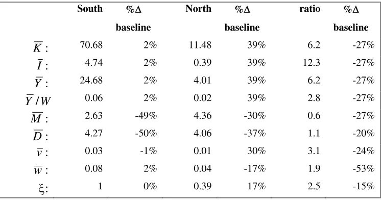
Scenario 3 – Defense Reductions

In this case we have both the North and South reduce their conscription rates and military

investment rates by 50%. This frees up both capital and workers for employment in the

production of goods and services. Table 4 shows the steady state values.

Increases are modest in the South. Output, production capital, military capital and

infrastructure rise by 2%. Unskilled wages fall by 1% and skilled wages rise by 2% across the

board

In the North output, production capital, military capital and infrastructure rise and become

39% higher than the baseline. Unskilled wages rise to 30% higher than the baseline while skilled

wages recover, though they still remain 17% below the baseline.

The steady state level of defense falls 50% in the South, but only 37% in the North. The

difference is due to the fact that there are much larger gains in productivity in the North than in

the South in the long-run, leading to relatively more military capital there.

6

Scenario 4 – A Free Trade Arrangement

In this scenario both the North and South retain their new lower levels of defense, but also

allow free trade in all intermediate goods with each other. Intermediate goods 1, 2, 6 & 7 are

still non-traded outside Korea. Prices of these goods must now adjust each period to ensure that

what is exported from one half the country is imported by the other half. Table 5 shows the

steady state values for this scenario.

Again, the gains from a free trade area are small, but nontrivial, in the South. Output,

production capital, military capital and infrastructure are 2% higher than the baseline. Skilled

wages, however, drop by an average of 24%. Given the South has a relative abundance of

skilled labor, the drop is not too surprising, but the size of the drop is quite large. A closer looks

shows that skilled wages in non-traded foods and natural resource extraction fall by over 60% of

their baseline values. These are the industries where the North actually has more skilled labor

and where the goods are not internationally traded, giving the North a comparative advantage

vis-à-vis the South. In the other two non-traded industries, utilities and non-traded services, the

South has a higher endowment of skilled labor and these wages rise to 17% above the baseline.

Skilled wages in the traded industries rise less than 1%. Unskilled wages also remain virtually

unchanged.

In the North we observe a symmetrical pattern with huge increases in skilled wages in

industries 1 & 2 (140% above baseline), and large declines in industries 5 & 6 (87% below

baseline). The movements in other skilled wages are smaller, but still large with a falling wage

in industries 4, 5 & 8 and a rising wage in industry 3. Output, production capital, military capital

and infrastructure rise an additional 21%. Unskilled wages rise 19%

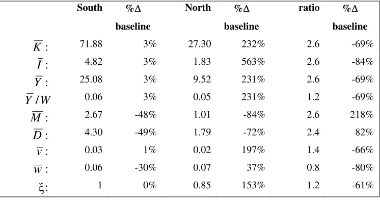
Scenario 5 – Common Economic Policy

This scenario requires a great deal more political cooperation than previous ones. It is hard

to imagine this occurring without some sort of political unification. We assume that the South

keeps its economic policies unchanged, but the North lowers its conscription rates and military

investment rates to the same levels as the South, while simultaneously raising the infrastructure

investment rate to also match the South. Table 6 show steady state values.

Not surprisingly, there are only small changes in the South’s steady state values. The only

substantial change is further movements in skilled wages. Falling in industries 1 & 2, and rising

There are huge movements in the North, however. Infrastructure quadruples, while output,

production capital and military capital double. Unskilled wages rise to 391% of the baseline and

the average skilled wage is 24% higher than the baseline..

The policy with the biggest effect, by far, is this one where the North reduces defense

spending and puts more into infrastructure.

Scenario 6 – Mobility for Skilled Labor or a Fully Integrated Economy

There is only one specific factor, skilled labor, for each intermediate good. If skilled labor is

allowed to migrate between the North and the South it will do so based upon the relative levels

of skilled wages in these two regions.

It is straightforward to show that the return on any particular type of skilled labor does not

depend on the amount of skilled labor employed as long as each sector is small. Intuitively, this

is because skilled labor is the unique factor which defines the industry. Capital and unskilled

labor are mobile across industries and the market will allocate them optimally across the

available skilled labor. If skilled labor were to expand in one small sector only, the market

would allocate a proportional increase in capital and unskilled labor to that sector. This would

have only an infinitesimal effect on the capital and unskilled labor in other sectors. Since we

have assumed constant returns-to-scale production this would lead to only infinitesimal changes

in marginal products of the factors leaving the equilibrium factor prices unchanged.

This means that allowing mobility of one kind of skilled labor only will not result in an

equalization of its wages between the North and South. Rather, all the skilled labor in that

particular industry would migrate from the low wage country to the high wage country, and the

skilled wage would remain unchanged.

If skilled labor of all types is allowed to migrate then factor prices will be effected since the

reallocation of capital and unskilled labor will no longer be infinitesimal. This means the

amount of skilled labor migration in any particular industry is indeterminate, but the total

migration of skilled labor of all types is uniquely determined. To resolve this indeterminacy we

assume that the percent of the total skilled labor endowment for the North and South actually

present in the South is the same for all industries. That is

i L L L

L L

L N

i S i N

i N i S i S

i =μ( + ); =(1−μ)( + ) ∀ (4.1)

c b c N N S S c b b N S c b b N S N f N f K K Z

Z + + +

− ⎟⎟ ⎠ ⎞ ⎜⎜ ⎝ ⎛ − − ⎟⎟ ⎠ ⎞ ⎜⎜ ⎝ ⎛ ⎟⎟ ⎠ ⎞ ⎜⎜ ⎝ ⎛ ≡ + = ) 1 ( ) 1 ( ; 1 1 ν ν ν

μ (4.2)

which is identical for all industries.

In the case where economic policy is the same in both the North and the South, technology

levels will be equal in the steady state. Both capital and skilled labor will be present in both

regions in the same proportion as the endowment of unskilled labor and all prices will be the

same as well. Thus, skilled labor mobility with identical economic policies amounts to the same

thing as a fully integrated economy, at least in the steady state.

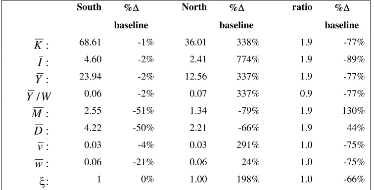
Table 7 shows a fully integrated economy. The location of production is indeterminate if

both types of labor are freely mobile across regions. For this table we assume skilled labor is

mobile, but that unskilled labor is not7. In this case, skilled labor will migrate out of the South

and into the North. We observe small drops in output, capital and infrastructure in the South. In

the North, we have increases in output, capital and infrastructure (on the order of 30%). The

average skilled wage falls by a third, and the unskilled wage almost doubles.

A Timed Phase-in of Reforms and Openness

Given currently political realities, it is difficult to predict what form unification of North and

South Korea would take. Unification could happen suddenly, as in the German case, with a

collapse of the political system in the North. It could also take the form of a military invasion.

We focus on a more gradual transition.

We imagine each of the previous scenarios occurring in succession with delays of five years.

Hence, we begin the simulation under the assumption of market reforms in the North. After five

years the North opens to trade with the rest of the world imposing tariff and non-tariff barriers

identical to those imposed by the South. After a further five years both the North and South

agree to cut military spending and conscription by half. In year 16, the North and South adopt a

free trade arrangement where intermediate goods from all sectors are freely traded across the

border, including those that are not currently traded internationally. Five years after this the

North adopts the same economic policy as the South. In year 26, migration of skilled laborers is

allowed, though unskilled laborers are not allowed to migrate. Finally, in year 31 we allow

unskilled workers to migrate as well. This leads to movements in technology levels through

7

congestion effects. As unskilled workers migrate from one region to the other, the effective level

of technology falls in the immigrant region and rises in the emigrant region such that unskilled

wages and technology are the same.

It is tedious, but straightforward to solve for the unique level of unskilled migration that

equalizes unskilled wage rates, which turns out to be the same as the migration rate for skilled

labor, μ.

) (

); )(

1

( N S S N S

N N N N N N

N = −μ + =μ + (4.3)

b h b b N S b h b h b N S K K I

I − − + − − − +

− − − ⎟⎟ ⎠ ⎞ ⎜⎜ ⎝ ⎛ ⎟⎟ ⎠ ⎞ ⎜⎜ ⎝ ⎛ ≡ +

= (1 )(1 ) (1 )(1 )

) 1 )( 1 ( ; 1 1 _ν ν

μ (4.4)

Since the capital to infrastructure ratio is not the same in both regions, the economy is not

fully integrated in the sense that the North and the South are not simply scaled versions of each

other. This is because capital and infrastructure accrue historically at different rates. However,

it is possible for the government to engage in infrastructure investment that equalizes the capital

to infrastructure ratios. Even if infrastructure investment is irreversible, this can be

accomplished via depreciation of the stock in one region and putting all new investment in the

other region. Since we are dealing with a single government (or at the very least, two highly

cooperative ones) we assume the government does this at the same time it allows unskilled labor

mobility. This gives us a fully integrated economy starting in period 31. We note that the

permanent sizes of the South and North will depend on the sizes of their respective capital stocks

in this period. This can be seen by reexamining (4.4) when the capital to infrastructure ratio is

the same in both regions.

) / ( 1 ) / ( N S N S K K K K + =

μ (4.5)

In our simulation this leads to large amounts of migration. This migration pressure could be

relieved by waiting longer to allow labor mobility which would lower the KS /KN ratio. Also,

the government could introduce taxes and subsidies in prior periods designed to encourage larger

capital buildup in the North and less capital buildup in the South.

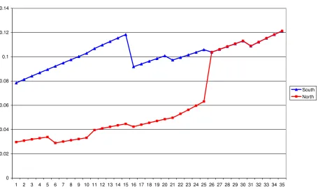
Figures 1 though 7 show the time path of various macroeconomic variables in the North and

South under this scenario.

Average skilled wages in the two regions equalize when skilled labor is allowed to migrate.

There is a large jump in skilled wages in the North when this happens. Skilled wages in the

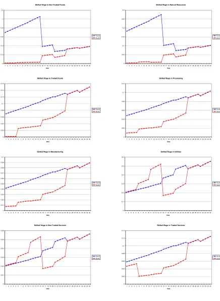
trade area. Figure 2 shows that the movements on specific skilled wages are very different from

the averages. For non-traded foods and natural resources (categories 1 & 2) the most dramatic

movements come with the free trade area, but skilled wages in the South remain higher than

those in the North until skilled labor migration is allowed. For utilities and non-traded services,

the drop in skilled wages associated with the free trade area occurs in the North, driving them

from levels above those in the South to levels well below those in the South. They rise

dramatically again when skilled labor migration is allowed. For all other industries (those where

there is significant trade with the rest of the world) skilled wages in the South respond very little.

In the North, they tend to rise with the implementation of the free trade area and again with

migration of skilled labor.

Figure 3 shows that unskilled wages rise in the South when skilled labor is allowed to

migrate. This is due to an influx of skilled workers into the South from the North which raises

the marginal product of unskilled labor. Equalization of unskilled wages due to migration of

unskilled labor then drives this wage down in the South and up dramatically in the North.

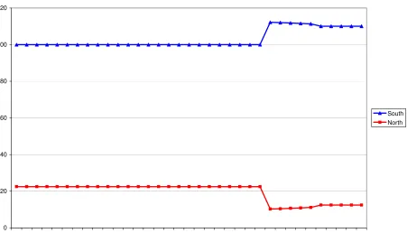
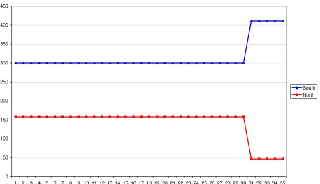
Figures 4 through 6 show that the movements in unskilled wages are driven primarily by

movements in levels of technology which are, in turn, driven by infrastructure congestion. When

unskilled labor is free to migrate, large numbers of unskilled workers migrate from the North to

the South, causing a drop in unskilled wages in the South and a rise in unskilled wages in the

North. This migration leads to infrastructure congestion in the South, lowering aggregate

productivity. The reverse is true in the North and aggregate productivity rises dramatically.

We assume in the scenario illustrated that there is no adjustment of the level of infrastructure

across regions. Instead, infrastructure per unskilled worker adjusts solely via unskilled labor

migration. The implied movements in unskilled labor are huge; more than two-thirds of the

North’s unskilled labor force moves to the South. This result is somewhat arbitrary. Since both

regions are simply scaled versions of each other, the government could just as easily choose to

invest more in the North’s infrastructure at the expense of the South’s. The amount of unskilled

labor migration needed to equalize unskilled wages would be smaller in this case.

Finally, table 7 shows that output per capita drops in the South and rises dramatically in the

North when unskilled labor is free to migrate. Again, this is due to technology jumps.

5 Conclusions

Our simulations indicate that the potential gains to North Korea from economic integration

great deal of uncertainty associated with our simulations. First, the parameterization of our

model (for North Korea in particular) is based on educated guess and assumption rather than

hard data. There is little that can be done about this other than to note the problem and perform

sensitivity analysis. Secondly, the timing of various reforms is speculative. We have no way of

knowing how much time would elapse between the North opening to international trade and

defense reductions, for example. They could well happen simultaneously. Policy makers are not

debating specific policies on infrastructure investment by the South in the North. Even the most

basic reforms we model seem unlikely in the near future.

With this important caveat, there is still a great deal of interesting behavior in the simulations.

We concentrate our attention on a few of the most important results.

First, adjustments to complete integration are likely to be large even with preparatory stages.

As we show, if there is no attempt made to equalize the levels of infrastructure per unskilled

worker, a majority of the North’s workers will want to migrate to the South. Undoubtedly much

of this is due to the simplicity of our model. There is no cost of migrating and the level of

technology depends strongly on the level of infrastructure per unskilled worker. Nonetheless, it

seems likely that unless the costs of migration were very high or technology was only very

weakly dependent on infrastructure per worker the amount of labor migration would still be very

high.

Second, the biggest long-run effects on output in the North come from changing government

policies. While movements in the direction of freer trade raise output per capita in the steady

state, the biggest gains come from raising infrastructure investment and lowering the defense

burden.

Third, the biggest effects on both skilled and unskilled wages in the North and South come

from allowing freer trade. This is either in the form of trade in goods or in the form of labor

migration. Hence, while overall welfare in the North is most strongly influenced by government

tax and spending policies, the biggest effects on owners of particular factors comes from the

References

Agénor, Pierre-Richard & Blanco Moreno-Dodson (2006) “Public Infrastructure and Growth: New Channels and Policy Implications,” World Bank Policy Research Working Paper 4064.

Albert, Max & Jurgen Meckl (1998) “Qualitatively Rational Expectations and Adjustment in the Specific-Factors Model,” Review of International Economics, vol. 6 no. 4, pp. 670-82.

Christiano, Lawrence J. (2002), “Solving Dynamic Equilibrium Models by a Method of

UndeterminedCoefficients,” Computational Economics, vol. 20, no. 1-2, pp. 21-55.

Eaton, Jonathan (1987) “A Dynamic Specific-Factors Model of International Trade,” Review of Economic Studies, vol. 54, no. 2, pp. 325-38.

Funke, Michael & Holger Strulik (2005) “Growth and Convergence in a Two-Region Model: The Hypothetical Case of Korean Unification,” Journal of Asian Economics, vol. 16 no. 2. pp. 255-79.

Kose, M. Ayhan (2002) “Explaining Business Cycles in Small Open Economies: 'How Much Do World Prices Matter?'”, Journal of International Economics, vol. 56 no. 2, pp. 299-327.

Noland, Marcus, Sherman Robinson & Ligang Liu (1999) “The Economics of Korean Reunification”, The Journal of Policy Reform, vol. 3 no. 3, pp. 255-299.

Noland, Marcus (2000) Avoiding the Apocalypse - The Future of the Two Koreas, Institute for International Economics: Washington, DC.

Roldos, Jorge E. (1991) “Tariffs, Investment and the Current Account,” International Economic Review, vol. 32, no. 1, pp. 175-94.

Shim, Ki R. (1993) “An Economic Model of Korean Reunification,” International Journal of Social Economics, vol. 20 no. 10, pp. 13-22.

Table 1

Total Trade as a Fraction of Sectoral Output, South Korea

Our Industries GTAP industries

1 Non-traded Foods 1 Paddy Rice 0%

2% 2 Wheat 3%

3 Cereal Grains 0%

4 Vegetables, Fruits & Nuts 3%

5 Oil Seeds 2%

6 Sugar Cane & Beets 0%

9 Livestock 1%

11 Raw Milk 0%

19 Beef 7%

22 Dairy 5%

2 Natural Resources 12 Wool 3%

5% 13 Forestry 3%

14 Coal 0%

18 Other Minerals 5%

3 Traded Foods 7 Plant Fibers 172%

61% 8 Other Crops 15%

10 Other Animal Products 22%

14 Fishing 35%

20 Other Meat Products 159% 21 Vegetable Oils & Fats 25%

23 Processed Rice 17%

24 Processed Sugar 192%

25 Other Foods 108%

26 Beverages & Tobacco 22%

4 Processing 27 Textiles 505%

191% 28 Apparel 187%

29 Leather Products 363%

30 Lumber 72%

31 Paper Products 59%

32 Refined Oil & Coal Products 270% 33 Chemical, Rubber & Plastic 181% 34 Other Mineral Products 34%

35 Ferrous Metals 143%

36 Other Metals 508%

37 Metal Products 109%

5 Manufacturing 38 Motor Vehicles & Parts 258% 310% 39 Other Transport Equipment 416%

40 Electronics 907%

41 Other Machinery & Equipment 135%

42 Other Manufactured Goods 163%

6 Utilities 43 Electricity 0%

0% 44 Gas Distribution 0%

45 Water Distribution 2%

7 Non-traded Services 46 Construction 0%

3% 52 Financial Services 2%

56 Public Adminstration 6%

57 Dwellings 0%

8 Traded Services 16 Petroleum N/A

26% 17 Natural Gas N/A

47 Trade 12%

48 Other Transport 22%

49 Water Transport 57%

50 Air Transport 210%

51 Communications 16%

53 Insurance 20%

Table 2

Parameterizations & Steady State for Baseline Model

Parameters

South North ratio

a1: 0.045 0.045 1.000

a2: 0.008 0.008 1.000

a3: 0.027 0.027 1.000

a4: 0.154 0.154 1.000

a5: 0.129 0.129 1.000

a6: 0.024 0.024 1.000

a7: 0.264 0.264 1.000

a8: 0.349 0.349 1.000

L1: 0.252 1.089 0.231

L2: 0.172 0.726 0.237

L3: 1.374 5.775 0.238

L4: 10.759 4.692 2.293

L5: 10.616 4.692 2.262

L6: 0.465 0.032 14.615

L7: 50.325 3.443 14.615

L8: 26.037 2.049 12.705

b: 0.441 0.441 1.000

c: 0.394 0.394 1.000

h: 0.5 0.5 1.000

gz: 0.015 0.015 1.000

β: 0.95 0.95 1.000

δ: 0.1 0.1 1.000

σ: 0.087 0.087 1.000

N: 300 157.5 2.222

f: 0.0418 0.124 0.337

m: 0.0245 0.25 0.098

i: 0.0221 0.01105 2.000

Steady State Values

South North ratio

ξ: 1.000 0.335 8.5

K : 69.608 8.228 16.9

I : 4.671 0.276 8.5

Y : 24.307 2.873 3.8

W

Y / : 0.061 0.016 0.8

M : 5.178 6.246 1.3

D: 8.490 6.415 1.0

r : 0.154 0.154 4.1

v: 0.033 0.008 36.6

1

w : 0.716 0.020 35.7

2

w : 0.187 0.005 32.4

3

w : 0.072 0.002 3.2

4

w : 0.049 0.016 3.3

5

w : 0.043 0.013 0.6

6

w : 0.207 0.358 0.6

7

w : 0.021 0.036 0.7

8

w : 0.060 0.081 1.7

P1: 0.303 0.177 1.7

P2: 0.242 0.142 1.7

P3: 0.207 0.124 1.1

P4: 0.195 0.171 1.1

P5: 0.190 0.166 0.9

P6: 0.247 0.286 0.9

P7: 0.169 0.196 0.9

Table 3

Steady State values for Scenario 2 - North Opens to International Trade

South %Δ

baseline

North %Δ

baseline

ratio %Δ

baseline

K : 69.61 0% 10.58 29% 6.6 -22%

I : 4.67 0% 0.36 29% 13.2 -22%

Y : 24.31 0% 3.70 29% 6.6 -22%

W

Y / 0.06 0% 0.02 29% 3.0 -22%

M : 5.18 0% 8.03 29% 0.6 -22%

D: 8.49 0% 7.69 20% 1.1 -17%

v: 0.03 0% 0.01 29% 3.2 -22%

w: 0.08 0% 0.04 -23% 2.0 -50%

ξ: 1 0% 0.38 13% 2.6 -12%

Table 4

Steady State values for Scenario 3 - Both North & South Lower Defense

South %Δ

baseline

North %Δ

baseline

ratio %Δ

baseline

K : 70.68 2% 11.48 39% 6.2 -27%

I : 4.74 2% 0.39 39% 12.3 -27%

Y : 24.68 2% 4.01 39% 6.2 -27%

W

Y / 0.06 2% 0.02 39% 2.8 -27%

M : 2.63 -49% 4.36 -30% 0.6 -27%

D: 4.27 -50% 4.06 -37% 1.1 -20%

v: 0.03 -1% 0.01 30% 3.1 -24%

w: 0.08 2% 0.04 -17% 1.9 -53%

Table 5

Steady State values for Scenario 4 – North-South Free Trade Area

South %Δ

baseline

North %Δ

baseline

ratio %Δ

baseline

K : 71.34 2% 13.68 66% 5.2 -38%

I : 4.78 2% 0.46 66% 10.4 -38%

Y : 24.89 2% 4.77 66% 5.2 -38%

W

Y / 0.06 2% 0.03 66% 2.3 -38%

M : 2.65 -49% 5.19 -17% 0.5 -38%

D: 4.29 -49% 4.59 -28% 0.9 -29%

v: 0.03 0% 0.01 55% 2.6 -35%

w: 0.06 -25% 0.03 -34% 1.8 -56%

ξ: 1 0% 0.43 27% 2.3 -21%

Table 6

Steady State values for Scenario 5 - Free Trade Area with Common Policies

South %Δ

baseline

North %Δ

baseline

ratio %Δ

baseline

K : 71.88 3% 27.30 232% 2.6 -69%

I : 4.82 3% 1.83 563% 2.6 -84%

Y : 25.08 3% 9.52 231% 2.6 -69%

W

Y / 0.06 3% 0.05 231% 1.2 -69%

M : 2.67 -48% 1.01 -84% 2.6 218%

D: 4.30 -49% 1.79 -72% 2.4 82%

v: 0.03 1% 0.02 197% 1.4 -66%

w: 0.06 -30% 0.07 37% 0.8 -80%

Table 7

Steady State values for Scenario 6 - Mobile Skilled Labor or Fully Integrated Economy

South %Δ

baseline

North %Δ

baseline

ratio %Δ

baseline

K : 68.61 -1% 36.01 338% 1.9 -77%

I : 4.60 -2% 2.41 774% 1.9 -89%

Y : 23.94 -2% 12.56 337% 1.9 -77%

W

Y / 0.06 -2% 0.07 337% 0.9 -77%

M : 2.55 -51% 1.34 -79% 1.9 130%

D: 4.22 -50% 2.21 -66% 1.9 44%

v: 0.03 -4% 0.03 291% 1.0 -75%

w: 0.06 -21% 0.06 24% 1.0 -75%

Figure 1

Average Skilled Wage

0 0.02 0.04 0.06 0.08 0.1 0.12 0.14

1 2 3 4 5 6 7 8 9 10 11 12 13 14 15 16 17 18 19 20 21 22 23 24 25 26 27 28 29 30 31 32 33 34 35

time

Figure 2

Skilled Wage in Non-Traded Foods

0 0.2 0.4 0.6 0.8 1 1.2

12 345 678 910 11 12 13 14 15 16 17 18 19 20 21 22 23 24 25 26 27 28 29 30 31 32 33 34 35

time

South North

Skilled Wage in Natural Resources

0 0.05 0.1 0.15 0.2 0.25 0.3

1 2345 678 910 11 12 13 14 15 16 17 18 19 20 21 22 23 24 25 26 27 28 29 30 31 32 33 34 35

time

South North

Skilled Wage in Traded Foods

0 0.02 0.04 0.06 0.08 0.1 0.12 0.14 0.16

1 2345 678 910 11 12 13 14 15 16 17 18 19 20 21 22 23 24 25 26 27 28 29 30 31 32 33 34 35

time

South North

Skilled Wage in Processing

0 0.02 0.04 0.06 0.08 0.1 0.12

1 2345 678 910 11 12 13 14 15 16 17 18 19 20 21 22 23 24 25 26 27 28 29 30 31 32 33 34 35

time

South North

Skilled Wage in Manufacturing

0 0.01 0.02 0.03 0.04 0.05 0.06 0.07 0.08 0.09 0.1

1 2345 678 910 11 12 13 14 15 16 17 18 19 20 21 22 23 24 25 26 27 28 29 30 31 32 33 34 35

time

South North

Skilled Wage in Utilities

0 0.1 0.2 0.3 0.4 0.5 0.6

12 345 678 910 11 12 13 14 15 16 17 18 19 20 21 22 23 24 25 26 27 28 29 30 31 32 33 34 35

time

South North

Skilled Wage in Non-Traded Services

0 0.01 0.02 0.03 0.04 0.05 0.06

1 2345 678 910 11 12 13 14 15 16 17 18 19 20 21 22 23 24 25 26 27 28 29 30 31 32 33 34 35

time

South North

Skilled Wage in Traded Services

0 0.02 0.04 0.06 0.08 0.1 0.12 0.14

1 2345 678 910 11 12 13 14 15 16 17 18 19 20 21 22 23 24 25 26 27 28 29 30 31 32 33 34 35

time

Figure 3

Unskilled Wage

0 0.01 0.02 0.03 0.04 0.05 0.06 0.07 0.08 0.09

1 2 3 4 5 6 7 8 9 10 11 12 13 14 15 16 17 18 19 20 21 22 23 24 25 26 27 28 29 30 31 32 33 34 35

time

Figure 4

Skilled Workers

0 20 40 60 80 100 120

1 2 3 4 5 6 7 8 9 10 11 12 13 14 15 16 17 18 19 20 21 22 23 24 25 26 27 28 29 30 31 32 33 34 35

time

Figure 5

Unskilled Workers

0 50 100 150 200 250 300 350 400 450

1 2 3 4 5 6 7 8 9 10 11 12 13 14 15 16 17 18 19 20 21 22 23 24 25 26 27 28 29 30 31 32 33 34 35

time

Figure 6

Technology

0 0.5 1 1.5 2 2.5

1 2 3 4 5 6 7 8 9 10 11 12 13 14 15 16 17 18 19 20 21 22 23 24 25 26 27 28 29 30 31 32 33 34 35

time

Figure 7

GDP per capita

0 0.02 0.04 0.06 0.08 0.1 0.12 0.14

1 2 3 4 5 6 7 8 9 10 11 12 13 14 15 16 17 18 19 20 21 22 23 24 25 26 27 28 29 30 31 32 33 34 35

time