http://dx.doi.org/10.4236/jmp.2016.76055
Coulomb Interaction in H2 Molecule for
States beyond the Ground State
Haiduke Sarafian
The Pennsylvania State University, University College, York, PA, USA
Received 16 February 2016; accepted 26 March 2016; published 29 March 2016
Copyright © 2016 by author and Scientific Research Publishing Inc.
This work is licensed under the Creative Commons Attribution International License (CC BY).
http://creativecommons.org/licenses/by/4.0/
Abstract
The focus of our investigation is to evaluate one of the four contributing terms to the coulombic potential energy of an H2 molecule. Specifically, we are interested in the term describing the elec-tronic interaction of the charge distribution of one of the hydrogen atoms with the proton of the second atom. Quantum mechanics provides the charge distribution; hence, the evaluation of this term is a semi-classic quantum physics issue. For states other than the ground state the charge distributions are not spherically symmetric; they are functions of the radial and the angular coor-dinates. For the excited states we develop exact analytic expressions conducive to the potential energies. Because of the functional complexities of the wave functions, the evaluation of the core integrals is carried out utilizing symbolic capabilities of Mathematica [1]. Plots of these energies vs. the distance between the two protons reveal global features.
Keywords
Coulomb Potential Energy, H2 Molecule, Excited States of H2, Symbolic Calculation, Mathematica
1. Motivation and Goals
Literature search reveals that quantum chemists customarily prefer adapting the shell method of charge distribu-tion of the electron calculating the coulombic related potential energy issues of an H2 molecule. In this method
one assumes that the charge distribution is composed of concentric spherical shells of finite thicknesses about the proton. Summing the potential contribution of the shells results in the total potential [2]-[4]. This method is a two-step process. Depending on the relative position of the point of interest to the center of the sphere one eva-luates the representative potential; then utilizing the latter one integrates over the radius of the atom. An alterna-tive intuialterna-tive method addressing the same issues is a volume charge distribution. Within the context of the H2
process and it is less cumbersome. As of our first objective in the analysis section we show the equivalency of these two methods. Our second objective is to adapt the latter method and craft an expression evaluating the electrostatic potentials of non-spherical charge distributions, i.e. distributions subject to states other than the ground state. The analysis section embodies one such expression enabling the evaluation of the potential of a desired excited state. In the course of derivation of this expression, because of the complexities of the wave functions we deploy the symbolic capabilities of Mathematica[1]. Our third objective is to utilize our derived formulation and for a handful of selected excited states explicitly evaluate their associated potentials. Plots of these results as a function of the inner-atomic distance between the two protons reveal certain characteristics; this is discussed in text. Lastly with concluding remarks, we close our investigation outlining our related conti-nual search.
2. Analysis
Following the objectives outlined in the previous section we consider the volume charge distribution method to evaluate the electrostatic potential of the charge distribution of a hydrogen atom. We consider two scenarios. First, we assume the distribution is confined within a sphere with a sharply defined radius R. For the case at hand the point of interest falls either outside or inside of the sphere; we will include more comments on this when we consider a diffused-edge sphere. We craft two distinct approaches evaluating their corresponding po-tentials. Second, because the charge distribution of the electron within the “sphere” according to the wave func-tion descripfunc-tion is diffused, we stretch the radius of the sphere harvesting the contribufunc-tion of the entire charge distribution. We show for the diffused ground state the volume and the shell charge distribution methods are equivalent. Next, for the excited states following the same strategy we modify the calculation to include the fea-tures of the non-spherical distributions. Utilizing this formulation for selective cases explicitly we evaluate their corresponding potential energies as a function of the inner-atomic distance.
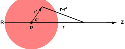
Figure 1 shows the charge distribution within a sphere of sharply defined radius R (the pink region); ρ
( )
ris the volume charge density, and r is the distance from the center of the atom. The coordinate system is set such that the proton is the origin and r is along the z-axis. The electrostatic potential at r is [5] [6],
( )
( )
1d
V =k ρ ′ ′
′ −
∫
r r r
r r (1)
where, k is the electrostatic constant k=1 4
(
π0)
. Since the z-axis is along the point of interest and r′ makesthe conic angle θ' with respect to the z-axis, expanding the denominator of the integrand gives,
[ ]
(
)
1 0
1
cos r
P
r θ
< + = >
′ =
′
−
∑
r r
(2)
where r< (r>) is the lesser (greater) of r and r', Pℓ, are the Legendre polynomials [5] [6]. For the ground state the
charge distribution is spherically symmetric; it is only a radial distance dependent function i.e.ρ(r'). On the oth- er hand the spherical volume element is 2
dr′=r′ sinθ′ ′ ′ ′d dr θ φd and that integration over the θ' gives,
(
)
π
0 0
cos sin d 2
l l
P θ′ θ θ′ ′ = δ
[image:2.595.204.423.612.698.2]∫
, i.e. only ℓ = 0 is non-zero. Utilizing this, for the points outside the sphere, combin-ing (2) and (1) yields,Figure 1.Charge distribution within a sphere of radius R.
Z r'
r r r'
' R
( )
( )( )
2 04π d
R
V r = K
∫
ρ r′ r′ r′ (3)For a special case of uniform charge density, (3) yields the classic expected potential V r
(
>R)
=Kq1r, where q is the total charge within the sphere. That is the potential of a uniform charge distribution for exterior points, it is the same as if the entire charge within the sphere was concentrated at the center of the sphere.Alternatively, one might omit the expansion given by (2) and directly integrate (1). To accomplish this, in (1)
we substitute r−r′ = r2+r′2−2rr′cosθ′; noting the ground state is independent of θ' and ϕ', a straight for- ward integration yields (3). Although this method works for the exterior points, i.e.r > R, it fails for the interiors,
r < R. For the latter we pursue the previous method; the details follow. By splitting the integration in two radial zones (1) reads,
(
)
( ) ( )
( )
( )
[ ]
[ ]
2 π
1 1
0 0 0
2π d d cos sin d
r R
r
r r
V r R K r r r r P
r r
ρ ρ θ θ θ
+
+ −
=
′
′ ′ ′ ′ ′ ′ ′
< = +
′
∑ ∫
∫
∫
(4)
In Formulating (4) we apply the previous assumptions, that the distribution is spherically symmetric. Noting the orthogonality of the angular integration mentioned earlier, i.e. 2δℓ0, (4) yields,
(
)
( )( )
2( )
0
1
4π d d
r R
r
V r R K r r r r r r
r ρ ρ
′ ′ ′ ′ ′ ′
< = +
∫
∫
(5) Assuming constant density, a straight forward integration of (5) yields,(
)
3 1 21
2 3
q r
V r R K
R R
<
−
= (6)
Equation (6) for r = R is the expected potential; its value matches the potential of the exterior on the surface of the sphere. The potential is continuous across the boundary of the sphere.
The intent of developing and reviewing this formulation is to evaluate the potential of charge distribution of an atom. Noting the distribution has a diffused boundary and because the radius of the “sphere” for a diffuse surface theoretically is infinite, the potential at any point needs to be evaluated according to (5).
For instance the charge distribution of the ground state of the hydrogen atom is
( )
( )
2 3100 8πe
r
e e
r q q α α
ρ = ψ r = −
where qe is the electron charge, α = 2/a and a is the Bohr radius, respectively [7]-[10]. Substituting ρ(r) in (5), a
straight forward integration gives the potential of the charge distribution as a function of distance r, the distance from the center of the atom. As discussed earlier to include all the charges of a diffused sphere we stretch the ra-dius of the sphere to "infinity", i.e. R→ ∞, this yields,
( )
1 11 e 1
2
r e
V r Kq r
r
α α
−
= − +
(7) This is the same as [2]. It is noteworthy to emphasize that contrary to our “volume charge distribution me-thod”, reference [2] adapted the “shell model” deriving (7). Having fulfilled the first objective of our goal i.e.
the proof of the equivalency of the volume vs. the “customary” shell distribution method, we adapt the latter and modify (5) to evaluate the potential of non-spherical charge distributions associated with the excited states. Needless to say, multiplying (7) by the charge of the second proton, qp, yields the attractive coulomb potential
energy of the electron-cloud of one of the atoms and the proton of the second atom in an H2 molecule.
For excited states of a hydrogen atom, density of the charge distribution is a function of {r,θ} and is indepen-dent of the azimuthal angle φ. It is,
( )
(
)
2( )
(
)
2, e NLM , , e NL LM ,
r q r q R r Y
ρ θ = ψ θ ϕ = θ ϕ (8)
here, RNL(r) is the radial wave function and YLM(θ,φ) is the spherical harmonics [8] [9] [11] [12]. Substituting (8)
( )
( ) ( )
( )
( )
(
)
(
)
(
[ ]
)
[ ]
2 1 2
1 1
0 0
2π π 2
0 0
1 1
2π d d
, cos sin d d
r
NLM NL NL
r
LM
V r K R r r r r R r r
r r
Y θ ϕ P θ θ θ ϕ
∞ +
+ −
=
′ ′ ′ ′ ′
= +
′
′ ′ ′ ′ ′ ′
×
∑
∫
∫
∫∫
(9)
In (9) although YLM’s are explicit functions of azimuthal angle φ’ their absolute squared are not; therefore, the
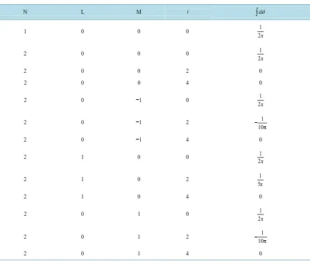
integral over φ' gives a factor 2π. The “orbitals” are labeled by N = 1, 2, 3, and the L's are bound to L=0,,N−1; this limits the number of potentials given by (9). Furthermore, for a chosen L, integration over the conic angle θ' limits the number of the terms in Σℓ. Table 1embodies the values of the integration over θ', for the
aforemen-tioned constraints. For a chosen L, Table 1gives the values and the number of the terms in Σℓ.
Inspecting Table 1reveals for a chosen excited state N and its associated L and M there are only a limited number of non-zero
∫
θ integrals. For instance, for the ground state{
N L M, ,} {
= 1, 0, 0}
there is only one [image:4.595.90.537.343.719.2]value for ℓ, i.e.ℓ = 0. For the first excited state
{
N M L, ,} {
= 2, 0, 0 and 2,1, 1}
{
±}
there are one and two values for ℓ; these are ℓ = 0 and ℓ = 0, 2, respectively. Table 1and its extension utilize the needed information asso-ciated with the remaining excited states. A careful inspection of this information shows, irrespective of the ex- cited state, only the even values of ℓ’s are conducive to non-zero∫
θ integrations.Table 1.A list of the first two excited states of hydrogen atom: N = 1 and 2 and their associated L and M as well as the ℓ’s
and the values of the integrals
∫
θ, respectively.N L M
∫
dθ1 0 0 0 1
2π
2 0 0 0 1
2π
2 0 0 2 0
2 0 0 4 0
2 0 −1 0 1
2π
2 0 −1 2 1
10π −
2 0 −1 4 0
2 1 0 0 1
2π
2 1 0 2 1
5π
2 1 0 4 0
2 0 1 0 1
2π
2 0 1 2 1
10π −
Applying (9) requires also knowing the explicit functional form of the radial wave functions. These functions are available in various references, e.g. [11] [12]. In our investigation and for Mathematica coding purposes we utilize a modified version of the code [13]. Table 2 displays various wave functions.
Table 2 embodies the first four radial wave functions of the hydrogen atom. It shows the complexity of radial
[image:5.595.91.539.353.720.2]wave functions of the excited states. Utilizing these functions along with their associated spherical harmonics we utilize (9) evaluating their corresponding electrostatic potentials. Table 3 embodies four such potentials.
Table 3embodies analytic expressions for the electrostatic potentials of charge distributions of the first five
states of a hydrogen atom. Similar to Table 2, complexities associated with these functions are evident. The simplest function corresponds to the ground state; as mentioned earlier this is in agreement with [2]-[4]. It is noteworthy mentioning that despite a thorough literature search, the author has not been able to locating a refer-ence referring to these expressions. Plots of these potential energies also are missing in the literature; these are shown inFigure 2.
Coulomb potential energies associated with various states of hydrogen atom are tabulated. The top left corner is the energy of the ground state. This is the same as discussed in [2]-[4] [7] [10]. These references have differ-ent mathematical approaches and do not include the graphs. The second row depicts energies of the first excited state. The third row illustrates the energies of the second excited state. These graphs are missing in the literature as well; they display useful information. For instance, they show how the excited states impact the electrostatic
Table 2. The first four radial wave functions of a hydrogen atom.
N\L 0 1 2 3
1 3 2 2e r a a −
2 2 ( )
5 2
e 2
2 2
r a a r
a − − 2 5 2 e 2 6 r ar a −
3
(
)
2 2
3
7 2
2e 27 18 2
81 3
r
a a ar r
a
−
− + 3 ( )
7 2
2
2 e 6
3 81
r
a a r r
a
−
− 3 2
7 2 2 2 e 15 81 r ar a −
4 ( )
3 2 2 3
4
9 2
e 192 144 24
768
r
a a a r ar r
a
−
− + − 4 ( 2 2)
9 2
e 80 20
256 15
r
ar a ar r
a
−
− + 4 ( ) 2
9 2
e 12
768 5
r
a a r r
a
−
− 4 3
9 2 e 768 35 r ar a −
Table 3. Coulomb potentials for the first five states of a hydrogen atom.
V100
2 2
e 2 1 e 2
r r
a a a r
ar − − + − V200
3 2 2 3
3
e 8 1 e 6 2
4
r r
a a a a r ar r
a r − − + − − − V210
5 4 3 2 2 3 4 5
3 3
e 96 1 e 96 8 7 e 22 6
8
r r r
a a a a r a a r a r ar r
a r − − + − + − + − − − V300 2 2
5 4 3 2 2 3 4 5
3 3
5
e 4374 1 e 2430 648 216 24 8
2187
r r
a a a a r a r a r ar r
a r − − + − − − + − V310
2 2 2
7 6 5 2 4 3 3 4 2 5 6 7
3 3 3
5 3
e 52488 1 e 34992 729 17 e 2997 540 72 6 2
729
r r r
a a a a r a a r a r a r a r ar r
a r
−
− + − + − + − − − − −
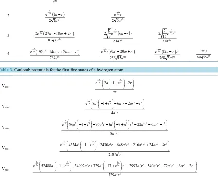
Figure 2.Plots of coulomb potential energies associated with excited states of a hydrogen atom.
energies. The functional behavior of these plots is somewhat intuitive, meaning, the excited states vs. the ground state are more spacious; therefore, they have a longer impact range. These are vividly shown by the tails of their associated energy plots. A quick review of these graphs also reveals that the energies of the excited states asso-ciated with PE210, PE310 and PE320 exhibit pronounced minima approximately at 1.2, 1 and 3.5 Å, respectively.
Our ongoing related investigation focuses on the physics of these minima.
Figure 3contains comparative plots of the potential energies. The left panel displays the energies of the first
three states of hydrogen associated with L = 0 states. The right panel similarly compares L = 1 energies of the second and third excited states. Both graphs show the energies associated with the excited states are stronger at short distances and coincide at large distances. Moreover, because the typical distance between two protons in an H2 molecule depending to their excited state is about 1 Å to 2 Å, at short distances the coulomb energies are
distinctly different. As shown on the right panel this distinction is more pronounced for L = 1 states.
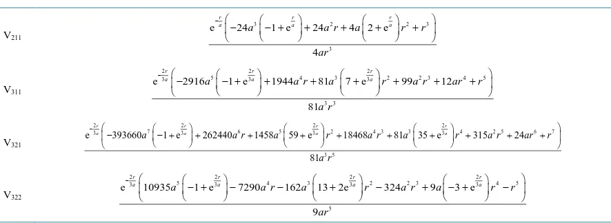
Table 4and Figure 4 are extensions of Table 3and Figure 2, respectively.Table 4 contains analytic
expres-sions for the second and third excited states of hydrogen. Figure 4 displays their corresponding potential ener-gies.
Tabulated energy plots of Figure 4have common general similarities vs. the plots ofFigure 3; the higher the excited states the weaker the corresponding energies. Contrary to the plots of Figure 2none of the energies dis-played in Figure 4exhibit pronounced minima. Accordingly, one may claim excited states circumvent the cou-lomb stability.
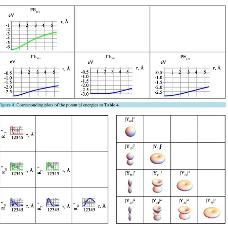
The left panel of Figure 5contains plots of the squared radial wave functions of the ground and excited states of the hydrogen atom. The right panel shows their corresponding plots of the absolute squared value of the spherical harmonics. These plots are visual components of Figures 2-4, respectively. To put this in prospective, (9) shows the squared of the radial wave functions and the squared absolute values of the spherical harmonics. As shown in Table 2, the integrands of (9) are complicated functions making the interpretation of the output challenging. However, with the aid of the displayed plots of Figure 5 one may reason the excited states are more spacious; they are radially stretched and are broadened. The impact of these two features on the potential ener-gies is signified by the long tails of the corresponding energy plots.
3. Conclusions and Comments
Motivation of proposing our investigation is to augment the current scope of energy issues of an H2 molecule.
Figure 3.Plots of potential energies of the L = 0 and L = 1 for the first three states of a hydrogen atom.
Figure 4.Corresponding plots of the potential energies to Table 4.
Figure 5. Plots of radial wave functions squared and their corresponding absolute squared spherical harmonics of various
Table 4. Coulomb potentials of the second and third exited states of a hydrogen atom.
V211
3 2 2 3
3
e 24 1 e 24 4 2 e
4
r r r
a a a a r a a r r
ar
−
− − + + + + +
V311
2 2 2
5 4 3 2 2 3 4 5
3 3 3
3 3
e 2916 1 e 1944 81 7 e 99 12
81
r r r
a a a a r a a r a r ar r
a r
−
− − + + + + + + +
V321
2 2 2 2
7 6 5 2 43 3 4 2 5 6 7
3 3 3 3
35
e 393660 1 e 262440 1458 59 e 18468 81 35 e 315 24
81
r r r r
a a a a r a a r a r a a r a r ar r
a r
−
− − + + + + + + + + + +
V322
2 2 2 2
5 4 3 2 2 3 4 5
3 3 3 3
5
e 10935 1 e 7290 162 13 2e 324 9 3 e
9
r r r r
a a a a r a a r a r a a r r
ar
−
− + − − + − + − + −
and potential energy associated with the charge distribution is a classic electrostatic problem. It is this semi- classic quantum physics nature of the issue that makes the problem appealing. Reviewing the sited references reveals that the majority of the investigations hover about the issues concerning the ground state charge distribu-tion of hydrogen. It is natural to augment the investigadistribu-tion extending the analysis to issues beyond the ground state. Mathematical analysis of our present work differs from customary quantum chemists. However, we show for the ground state we are in agreement. Having established the equivalency of these two approaches we extend the formulation to consider states beyond the ground state. Because of the analytic complexities of the expres-sions we adapt the symbolic capabilities of Mathematica generating explicit analytic functions for the potential energies. Our work includes fresh graphic information not reported in various literatures; it puts the formulation to perspective. Currently we are extending the investigation to include electrostatic energies corresponding to the electron cloud-cloud interaction. Although this issue has been already investigated for the ground state con-figuration, there is no complete formulation to include the excited states. Pursuing our new initiative thus far, we have realized the complexities of the mathematical challenges. The author doubts that the electron exchange term of the coulomb energy of the excited states will ever be solved analytically!
Acknowledgments
A version of this investigation was presented at the ATINER International conference, Athens, Greece, July 2015.
References
[1] A Symbolic Mathematical Computation Program, V10.3, 2015.
[2] Pauling, L. and Wilson, E.B. (1963) Introduction to Quantum Mechanics with Applications to Chemistry. Dover Pub-lications, Inc., New York.
[3] Kauzmann, W. (1957) Quantum Chemistry, an Introduction. Academic Press Inc., New York.
[4] McGlynn, S.P., Vanquickenborne, L.G., Kinoshita, M. and Carroll, D.G. (1972) Introduction to Applied Quantum Chemistry. Holt, Rienart and Winston, Inc., New York.
[5] Jackson, J.D. (1999) Classical Electromagnetic. 3rd Edition, John Wiley, New York.
[6] Arfkin, G. (1968) Mathematical Methods for Physicists. Academic Press, New York. [7] Davydov, A.S. (1966) Quantum Mechanics. NEO Press, Ann Arbor, Michigan.
[8] Powell, J.L. and Crasemann, B. (1965) Quantum Mechanics. Addison-Wesley Company, Inc., Boston. [9] Schiff, L. (1968) Quantum Mechanics. 3rd Edition, McGraw-Hill Book Company, Tokyo.
[10] Wallace, P.R. (1984) Mathematical Analysis of Physics Problems. Dover Publications, Inc., New York.
[11] Beth, H.A. and Salpeter, E.E. (1977) Quantum Mechanics of One- and Two-Electron Atoms. Dover Publications, Inc., New York.
[12] Flugge, S. (1974) Practical Quantum Mechanics. Springer-Verlag, New York.