Reliability Control for Aggregation in Wireless Sensor Networks

Reliability Control for Aggregation in Wireless

Sensor Networks

Jonathan P. Benson, Tony O’Donovan, Cormac J. Sreenan.

Mobile and Internet Systems Laboratory (MISL),

Computer Science Department, University College Cork (UCC), Ireland

—

Utz Roedig

InfoLab21, Lancaster University, UK

Abstract— Data aggregation is a method used in sensor networks to reduce the amount of messages transported. By aggregating, the data contained in several messages is fused into one single message. If such a message, containing the equivalent of many individual messages, is lost due to transmission errors then this has a detrimental effect on the application quality experienced. In many sensor network applications a constant supply of data is needed and therefore application quality is severely effected by excessive data loss. This paper proposes and evaluates the use of an in-network control mechanism to offset this disadvantageous effect. The control mechanism analytically calculates the correct reliability that an aggregate of given size must be forwarded at in order to meet application specific goals.

I. INTRODUCTION

Many wireless sensor network (WSN) applications collect periodically generated sensor data at a central point - the data sink or base station - where the data is subsequently analysed. This class of applications is considered within this paper.

In a realistic deployment scenario, messages are lost in transport while travelling hop-by-hop through the network towards the sink. These packet losses happen due to the natural lossy characteristics of the wireless links between the sensor nodes. An application analysing the data may be able to deal with some of these losses. More specifically, the application might be able to infer the correct conclusions even if a (small) portion of the sensor readings is not available for the analysis. This could be due to the ability to interpolate missing data or the availability of redundant sensor data.

Using data aggregation, several messages transported along the same path can be combined into a single message. Aggregation techniques reduce the amount of messages and thus reduce energy expensive transceiver operation and help to preserve scarce bandwidth. As aggregation increases the amount of data concentrated in a single message, the data reliability at the sink is altered. Losing a message containing a single data reading has surely a different impact on the overall data reliability than losing a message containing the information of several sensor readings. This effect is described in [11]. Where aggregation occurs the average amount of data arriving at the sink, expressed by the expected valueE(X)is unaltered compared to when aggregation is not used. However

this has the effect of increasing the variance about E(X)

and therefore the standard deviationσ. This leads to unstable application quality since the amount of data arriving at the data sink can fluctuate significantly.

This paper presents and evaluates a control mechanism to combat the effects of the increases in σ caused by in-creasing amounts of aggregation. Worst case dimensioning was examined in [11] where it was found that, although the methods used were successful from a dimensioning point of view, significant overshooting of application defined targets occurred due to the use of worst case assumptions. In contrast this paper relaxes the assumptions used and recalculates the necessary forwarding reliability to meet application targets as aggregation occurs in network. This offers a much more fine grained approach than [11] and also relaxes a number of assumptions used in that paper. An alternative to altering the forwarding reliability to suit the aggregation level would be to adjust the aggregation level to suit the inherent reliability of the links available. However, the number of assumptions necessary for this approach are far greater than those for the method examined in this paper. In addition it is easy to see a situation arising whereby, without global knowledge of network condi-tions, aggregated data may need to be broken up and reformed as it progresses through the network and encounters different conditions. Therefore modifying the aggregation level to suit the link reliabilities found is not considered in this paper.

The remainder of the paper is organised as follows. Section II describes the motivation for this work. Section III discusses related work. Section IV analyses the effects of aggregation while section V describes how our control goals are formally set. Section VI describes how this goal is achieved. An ex-perimental evaluation of the control methodology is presented and examined in section VII. Finally conclusions and future work are discussed in section VIII.

II. MOTIVATION

detected. In contrast another class of applications periodically gather data from the sensor network and use this data for a particular purpose (It is this class of applications under consideration in this work). In some cases this data may be for the purposes of logging a phenomenom while in others some form of control or actuation may take place based on the data collected. In the case of actuation or control data must be successfully delivered in sufficient quantity to ensure the application can function correctly. The tolerance to lost data will be defined by the nature of the application, the degree of redundant sensors available and the ability to interpolate missing data. Consider the following scenario. An industrial cooling system consists of a large lattice of pipes which deliver pressurised coolant to nozzles which spray the coolant onto a surface below. Each of the nozzles must deliver the correct amount of coolant and a network of sensors monitors the pressure in the pipe lattice feeding the nozzles. A drop in pressure in a pipe means that remedial action needs to be taken and pressure is restored by closing relief valves or by increasing the pressure of the input feed to that section of pipe. In this scenario data must regularly be delivered to the application and any data loss must not exceed application defined tolerances (i.e. there are redundant sensors in each section of the lattice).

For the purposes of this study an application similar to the one outlined above which periodically gathers sensor data from the network (or a particular region or subsection of the network) is considered. Within each data gathering interval each sensor generates a reading which is transmitted to the data sink. It is worth stating that the use of data gathering intervals does not suggest that fine grained time synchronisation is needed. Nodes can generate and send data in a periodic manor based on the time of arrival of an interest. The sensor readings generated may or may not be aggregated en route to the data sink. Due to the lossy nature of the wireless channel several messages will inevitably be lost. How this loss affects the application quality is described below.

A. Data Reliability and Application Quality

It is assumed that the needs of an application analysing data at the sink of a sensor field can be given by a utility function. Consider a simple utility function U(X) for some arbitrary application.U(X)is a function of the percentage of the total amount of sensor samples sent that the application receives during a discrete time interval. The utility function indicates how useful a certain amount of data units are to an application and is thus a mapping of application level quality requirements to data transport reliability. At some point the required amount of sensor samples are received that will give an acceptable utility value. It has to be noted that simple utility functions cannot be used for all application types. For example in cases where the data readings of specific sensors are more important for the functioning of the application than others. However, a large class of data gathering applications can be described by utility functions.

If the quality of the application depends on the amount of

received data as it is described by the utility curve, a mapping between data delivery reliability and application quality is possible. The amount of data being delivered during each time interval has to be kept at a value such that the utility of the application is kept at an acceptable level. The variance in the amount of data delivered has to be controlled also since fluctuations below the minimum amount of data required would prevent the utility from staying at a constant acceptable level. Thus, if the utility curve of an application is known, the bounds for the minimum amount of data per discrete time interval can be determined and the correct reliability measures can be put in place in order to facilitate the correct operation of the application.

III. RELATEDWORK

The related work section is split into two parts that discuss previous work related to the research presented in this paper. First, related work on data aggregation in sensor networks is discussed. Second, existing work that describes methods to control the reliability is presented. Reliability control is the method proposed in Section VI to counter the problem of variable link reliability and path length; thus it is important to show that appropriate technical implementations exist.

1) Aggregation: Several papers address the issue of ag-gregation in sensor networks. These papers vary in their approaches and emphasis.

A common approach is to abstract aggregation from the underlying network operation by implementing a SQL like query layer which a programmer or end user can use to pose queries to the sensor network [1], [2], [3], [4]. It is arguable whether some of the functions of query based aggregation are in fact aggregation. Often the function of SQL-like queries is to filter data and reduce the number of tuples rather than actively use and combine data into an aggregated format. MIN and MAX operators are examples of such functions. This form of aggregation is not related to the problem discussed within the paper. In this paper is assumed that the application requires a minimum number of sensor samples to derive a correct decision. This assumption allows a more generalised view of aggregation methods and allows for redundancies inherent in sensor networks.

Other related work considers that sensors can only detect a phenomenon with limited accuracy [12]. This uncertainty in the sensor readings can be interpreted as detection relia-bility. If several sensors monitor the same phenomenon, this uncertainty can be mitigated. This spatial and/or temporal correlation of sensor readings can also be used for aggregation purposes in the network [13]. Normally the reduction of sensor reading uncertainty can be traded for the aggregation level [14]. Methods to improve sensing accuracy in conjunction with aggregation are not investigated in this paper.

approach is to forward a message more than once so that its reliability is increased [7], [8], [9]. A more complex method involves forwarding multiple packets along multiple disjoint paths [7], [8], [9]. The loss/corruption of data packets due to noisy wireless channels and data errors, and a method to correct this corrupt data are investigated in [15]. [10] is closely related to this work in a number of respects, although aggregation is not the focus, and describes, in general terms, some methods that may be used to evaluate the informational value of sensor data. Various informational values are then mapped to various protection measures, FECs (Forward Er-ror Correction codes) in this case. The principal difference between that paper and this is that this paper presents a formal link between data and the reliability needed for a given application scenario. [10] does not calculate the required reliability for an aggregate and does not take into account the number of hops to the data sink.

IV. AGGREGATION- RELIABILITYINTERDEPENDENCY

This Section defines the terms aggregation and data trans-port reliability. Subsequently, the interdependency between data transport reliability and data aggregation is investigated.

A. Aggregation

The term data aggregation, sometimes also referred as message aggregation, can be applied to a range of different operations taking place inside a network. For the purposes of this study, a valid aggregation functionφis defined as follows:

Definition 1: An aggregation functionφmaps several

mes-sages to a single message. Formally, if M is the set of all possible messages transmitted, this can be expressed as:

φ: Ma _{→M ∀a≥2.}

Data aggregation is used in sensor networks for several rea-sons. The main objective of data aggregation is the reduction of energy consumption. Energy is saved as less messages, normally containing a smaller payload than the unaggregated messages together, have to be forwarded. An additional effect of aggregation is the reduced amount of bandwidth necessary to transport information through the network.

There are several approaches to data aggregation which can be used on their own or in combination. On a packet level it is possible to combine the payload of several messages in a single message. This form of aggregation leads to energy savings as the header overhead is reduced, energy costly media access mechanisms have to be executed less frequently or the hardware defined fixed frame capacity is used efficiently. A different aggregation approach consists of applying in-network functions to process or pre-process the data generated. These functions include SQL type operators such as SUM, AVG, COUNT and combinations thereof. Other more application specific functions may be possible to implement in-network. These may include data correlation, correction and verification algorithms or data fusion algorithms. In general, if the infor-mation required from the sensor network is a functionf such thatf(x1, x2, x3) =f(f(x1, x2), x3) =f(x1, f(x2, x3))then

the result can be computed in parts as data is transferred in the

network towards the base-station. This form of aggregation is applied on the application level and leads to energy savings as the net amount of bytes transmitted is significantly reduced.

B. Reliability

In this paper, it is assumed that sensor data readings are transported towards a sink. It is assumed that all sensor samples are considered to be equally valuable. It is generally difficult to ascertain the “value” of a given sensor reading with respect to another and it is more difficult to ascertain the correct value of an aggregate of a number of such sensor readings. One method of evaluating aggregates is to simply count the number of sensor reading contained therein. It can be argued that this method is inappropriate for evaluating a number of query based aggregates. For example, when using the MAX operator the most valuable sensor reading, whether a part of an aggregate or not, is the one with the highest value at that given time or during a specific time interval. However it can be argued that MAX, MIN and similar functions should be disregarded as they are actually data suppression or filtering functions as opposed to aggregation functions which combine data.

A further assumption is that a collisionless TDMA-like MAC protocol is used and as a consequence error rates are traffic invariant. We believe that these assumptions still result in a reasonably accurate model that can be used for the study described in the paper. Using the assumptions, the reliability on the different abstraction levels is given by the following three definitions:

Definition 2: The hop-by-hop message transport reliability (short: hop-by-hop reliability), rij, describes the probability that a message is delivered successfully between two neigh-bouring sensor nodesi andj.

Definition 3: The end-to-end message transport reliability (short: end-to-end reliability),r, is described by the product of the message transport reliabilitiesri,j on the path from source to sink.

Definition 4: The data transport reliability (short: data reli-ability) is described by the expected amount of sensor readings

E(X)per unit time reaching the sink and also by the variance

σ2

. The variance describes fluctuations about the expected value.

C. Interdependency

The data reliability, characterised by E(X) and σ2

, is influenced by the amount of data lost in transit. These losses are characterised by the hop-by-hop reliability of each link and the degree of aggregation. The degree of aggregation,a, influences how many data readings are lost by losing a single message.

Consider a line of nodes where the topmost node is the data sink and the bottommost node has a number of N

unaggregated asN messages, each containing a single sensor reading, or aggregated in n ≤ _N messages depending on the selected aggregation degree. The value 1 ≤ _a ≤ _N

describes how many readings are combined in each message. Thus it is assumed that all messages carry the same number of

a sensor readings (homogeneous aggregation). Note that the assumption of homogeneous aggregation has no net effect on the expected value calculations and gives a worst case variance calculation for a maximum aggregation levela. As a result of the aggregation, the following number of messages are sent to the sink:

n=N/a (1)

1) Expected Values : The question here is how aggregation influences the expected value E(X). The expected value can be calculated by:

E(X) =

n

X

a·r=n·a·r (2)

Using (1) and substituting the value ofawithN/ngives:

E(X) =N r (3)

Thus, the expected value1 is a function of the number of sensor data N and the end-to-end reliability r. The degree of aggregation a has no effect on the expected value. It therefore seems logical to aggregate as much as possible as no cost regarding data transport reliability, in terms of the expected value, must be paid. In the literature it is sometimes, for example [10], assumed that aggregated packets should be handled with greater care than non-aggregated ones. As shown, this is not true regarding the expected value of the amount of data readings.

2) Variance: The variance gives an impression of the fluctuations of the amount of data readings reaching the sink. The varianceσ2

is given by the formula:

σ2

=E(X2

)−_[E(X)]2

(4)

The variance can now be calculated and using (1):

σ2

=

n

X (a2

·r)−(a2

·r2

) =N·a·r·(1−r) (5)

Here, the variance depends linearly on the degree of ag-gregation and linearly on the number of samples. Now both extremes can be compared; no aggregation with a = 1 and total aggregation with a=N. In the first case, the variance depends linearly on the amount of sensor readings. In the second case, the variance depends quadratically on the amount of sensor readings sent. It can be concluded that the variance of amount of data readings per time unit reaching the sink depends heavily on the degree of aggregation. Regarding the variance it is therefore useful to handle aggregated packets with greater care than non-aggregated ones.

1_{The equations used here are used for simplicity and brevity. Probability} of delivery of data packets has a binomial distribution. Expected values for binomial probabilities can be reduced to give the same result.

V. AGGREGATION- RELIABILITYCONTROL

In this Section, the control goals are formulated along application requirements. Thereafter the control mechanism and its implementation is presented.

A. Application Requirements

It is assumed that an application requires a data transport reliability above a given value to function correctly. Mathe-matically expressed, it is required thatE(X)≥N ·R. Here,

R is the reliability level desired by the application,N is the total number of sensor data. Additionally, it has now to be taken into account that the amount of actual data delivered will fluctuate about the expected value, which is described by the variance. Thus the control goal is defined as:

Definition 5: The network should achieve a transport reli-ability such that expected value minus some multiple of the standard deviation equals to or is greater than the minimum re-liability level desired by the application. This can be expressed as follows:E(X)−_{zσ >=N R}.

For example, if a normal distribution of the incoming sensor readings is assumed and z = 1.96 is selected, in 97.5% of cases the application requirements can be met.

B. Control Mechanism

As it was shown by (3) and (5), the expected value and variance depend on the aggregation degree a and the end-to-end message reliability r. Thus, aggregation degreea and end-to-end transport reliability r have to be balanced, such that the needs of the application can be met.

Using the application requirements given in Definition 5, equations that allow the computation of the maximum aggre-gation degree and/or the necessary transport reliability can be derived:

E(X)−N R=zσ (6)

Using (2) and (5):

n·a·r−N·R=z·pN·a·r·(1−r) (7)

Squaring both sides of (7) gives:

N2

·(r2

−2·r·R+R2

) =z2

·N·a·r·(1−r) (8)

To calculate the maximum aggregation degree a if r is already known, (8) can be modified as:

a=N·(r

2₋

2·_r·_R+R2

)

z2_·r·(1−r) (9)

Finally the following equation to compute the end-to-end transport reliability r needed for a givena can be generated using (8):

(N+z2

·a)·r2

−(2·N·R+z2

·a)·r+N·R2

Equation (9) gives the maximum aggregation degree that can be used in the network if the end-to-end reliability r

is known. Solving (10) for r gives the necessary end-to-end reliability for messages if the aggregation degree is known. Of course, both equations can be used together to balance these values.

C. Reliability Control

Equations (9) and (10), assume that the end-to-end relia-bility, r, for messages transported in the network is constant for all messages regardless of their distance to the sink. For example, if a constant hop-by-hop reliability is assumed, mes-sages will have a different end-to-end reliability. A possible solution to this problem and one which is explored in this work is to ensure that all messages achieve the same end-to-end reliability r. The method used to do this is described in Section VI-A.

VI. CONTROL METHODOLOGY

In order to consider the use of a dynamic in-network solution without the use of global knowledge it is necessary that the individual actions of the nodes lead to the desired goals. In order to see that this is true consider the following:

Fact 1: E(X) = Σ(Xi)

Fact 1 merely states that the overall expected value is merely the sum of all the expectancies within the network. For example if one message has an expected value of 0.7 and another an expected value of 0.8 then their combined expected value is 0.7+0.8=1.5

Fact 2: σ2

= Σσ2

i

Fact 2 states that the variance is the sum of the individual variances from within the network. This holds since the delivery probability of each message both uncorrelated and independent. If this is the case then

var( n

P

i= 1 Xi) =

n

P

i= 1

var(Xi)

If both fact 1 and 2 hold then the following must hold also.

Fact 3: If E(Xi)−σi=Ri then

N

P

i= 1

(E(Xi)−σi) =E(X)−σ=N R

This means that if techniques to modify the reliability to meet the condition described by (6) are applied within the network, global awareness is not necessary in order to satisfy (10).

Equation (10) can therefore be modified to determine the correct end-to-end reliability for any given aggregate. To do this (10) is simply divided byato give:

(N a +z

2

)·r2

−(2·N

a ·R+z

2

)·r+N a ·R

2

= 0 (11)

A. Adaptation

Each node must know the number of reporting nodes N. This information will be monitored at the data sink and disseminated via requests along with the desired reliabilityR. Using this data each node will then compute the correct end-to-end-reliability r needed for a packet or aggregate packet using (11).

A node adapts its forwarding mechanism such that the desired end-to-end reliability r for the message is achieved. A node, upon receiving a request from the data sink to generate messages and forward these messages with end-to-end reliabilityrwould need to know the number of hopshto the data sink (it is assumed that the routing tree is stable). The node could then calculate the reliability rf at which it would need to forward this message over each hop to meet the end-to-end reliability requirements. To calculate rf the following simple formula is used: rf = ceiling(loghr). The value of

rf needs to be forwarded in each packet so that the receiving node is able to calculate what steps it needs to take to ensure that the packet is again forwarded with reliabilityrf. Methods to achieve the desired rf are discussed in the III section. In particular, [7], [8], [9] discuss this in detail.

Consider the following example:

• Node A receives two packets from different senders which are to be aggregated. Node A needs to calculate the end-to-end reliability,r, necessary for a packet consisting of two data samples. Node A does this using (11).

• Using r and the number of hops to the data sink the required forwarding reliabilityrf can be calculated.

• Now node A must examine the forwarding reliability constraints in both of packets containing the data to be aggregated. Let us call them rf1 and rf2 respectively

and denote the forwarding reliability calculated in the previous step as rf a (a denotes aggregate). The final forwarding reliability, rf, is simply max(rf1, rf2,rf a). Note that the effects of ignoring this step is examined in Section VII-D.

• Having calculated rf the amount of retransmissions, redundant packets or other reliability measures needed to achieve this reliability level (assuming the link error probability is known) must be calculated.

VII. EXPERIMENTALEVALUATION

A. Topology

100nodes are placed in a grid. The transmission range is set such that each node can only communicate to their adjacent neighbours in the grid. The topmost left node is designated as the data sink and the other 99 nodes deliver data to this location. A request is flooded by the sink into the network and a routing tree is formed along the reverse path. For the purposes of the experiment the routing tree is considered to be stable.

B. Aggregation

its upstream neighbours. Since the envisaged operation of the sensor network in this paper is periodic a cascading system can be put in place. In such a system each node will wait for a progressively longer period as hop distance to the data sink decreases. This allows adequate time for data generated from nodes farther away to catch up and be aggregated. The method is formally described as follows: A waiting periodTi at nodeni,hi hops from the data sink, in the routing tree is calculated for each message in order to facilitate a cascading aggregation system using the following formula:

Ti=

Tmax

hmax

·_(hmax−_hi)

It is assumed thatTmax<data gathering interval.

C. Traffic

Every node periodically generates a sensor reading (1 per sensing period) and sends it to the data sink. Before the next period all the data generated is forwarded to the sink and recorded. Each node generates 1000 data readings per simulation. After each period the amount of sensor readings delivered to the sink is recorded. Finally the standard deviation is calculated for the 1000data gathering rounds.

Rather than set the maximum aggregation level a or cal-culate a worst case scenario forwarding reliability rf (as was done in [11]) the end-to-end and forwarding reliability is re-evaluated when aggregation occurs in the network. This should reduce the amount of overshooting seen in [11]. Aggregation is allowed to grow without bound and packet size does not increase except in later experiments in section VII-F where the effects of growing packet size on the number of retransmissions needed is examined.

The experiments use a simple bit error model and it is as-sumed that each node has an accurate bit error rate estimation (the effects of inaccuracies in the BER estimation is examined in section VII-E). Naturally acknowledgements are also prone to errors. The basic calculation for converting bit error rates (BER) to packet error rates (PER) and acknowledgement error rates (AER) is given by the following formula: P ER or

AER = (1 −_BER)length _{where length is the length of} the packet in bits. No correctable bits are assumed. A fixed packet length of 160 bits (20 bytes) and 80 bits (10 bytes) is assumed for data packets and acknowledgements respectively, except in the case where packet length is allowed to grow with aggregation. Given the assumption that the link reliability can be modified a mechanism to do so must be provided. The cho-sen mechanism in these experiments is an ARQ protocol. The number of retransmissions needed is calculated using the fol-lowing formula:max transmissions=ceiling(logP ER(r)). Naturally the rounding upward, to a whole number, of the number of transmissions to be used results in a small amount of overshooting of the target reliability.

D. Experiment 1

The dynamic control methodology is implemented and tested for a variety of differing target reliabilities ranging

0 20 40 60 80 100

0 0.2 0.4 0.6 0.8 1

Data Recieved [%]

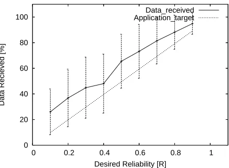
Desired Reliability [R] Data_received Application_target

Fig. 1. Algorithm performance with end-to-end constraints.

0 20 40 60 80 100

0 0.2 0.4 0.6 0.8 1

Data Recieved [%]

Desired Reliability [R] Data_received Application_target

Fig. 2. Algorithm performance without end-to-end constraints.

from 0.1 to 0.9. Packet sizes are fixed and do not grow due to aggregation. A constant bit error rate of 0.002 is used which gives a packet error rate (PER) of 0.247 and an acknowledgement error rate (AER) of 0.148.

Two separate experiments were run. The first kept the constraints set by packets sent from further away (highestrf, discussed in section VI-A) while the second experiment did not. In addition the results of these experiments are compared in two different ways. Firstly the average amount of data delivered is examined with the standard deviation shown as error bars. Secondly the amount of failed data rounds (where the data delivered was less than70%) is considered. Since a z-value of 1.0 is used this implies that 85.13% of rounds should be successful. In essence figures 1 and 3 are from the same data and likewise with figures 2 and 4 represent the second experiment.

20 30 40 50 60 70 80 90 100 110

0 0.2 0.4 0.6 0.8 1

Successful Rounds [%]

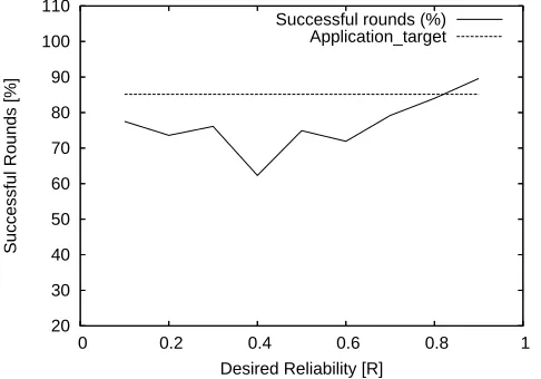
Desired Reliability [R] Successful rounds (%)

Application_target

Fig. 3. Number of failed rounds of data gathering with end-to-end constraints.

20 30 40 50 60 70 80 90 100 110

0 0.2 0.4 0.6 0.8 1

Successful Rounds [%]

Desired Reliability [R] Successful rounds (%)

Application_target

Fig. 4. Number of failed rounds of data gathering without end-to-end constraints.

it can be seen that in excess of the target 85.13% of data rounds were successful in every case. When ignoring end-to-end constraints, figure 2, it can be seen that the average data received tracks the desired reliability R more closely although the standard deviation invariably fails to come within target in every case. An examination of figure 4 reveals that the required amount of data is rarely received where end-to-end constraints are not kept, indicating it is necessary to keep the constraints. Thus there are two reliability constraints that an aggregate must obey; those derived from (10) and the maximum forwarding reliability of all the constituent messages. However adopting the most conservativerf results in a significant amount of over shooting the target reliability which can be seen in both figure 1 and 3. This is due to the fact that aggregates must become reasonably large before the increase in reliability necessitated by increased variance exceeds the maximum forwarding reliability of the worst case hop distance. Thus many aggregates get a “free” boost in their end-to-end reliabilities by aggregating with data that is further from the sink. Also note that the rounding up of the number

0 20 40 60 80 100

0 0.0005 0.001 0.0015 0.002

Data Recieved [%]

BER randomness

Data_received Application_target

Fig. 5. The effect of fluctuations in the BER on reliability

60 70 80 90 100 110

0 0.0005 0.001 0.0015 0.002

Successful Rounds [%]

BER randomness

Successful rounds (%) Application_target

Fig. 6. The effect of fluctuations in the BER on reliability

of transmissions used contributes to this overshooting. While this is not ideal from an analytical perspective it does allow a relaxation of assumptions such as accuracy of BER estimation which shall be see in the next experiment.

E. Experiment 2

One weakness that is present in the methodology chosen is that it is reliant on the accuracy of the bit error estimation process available to the sensor node. Naturally this estimation may not be entirely accurate and errors and fluctuations will cause some variance from this figure. This experiment introduces a randomly generated value, of varying range (±0.0002, 0.0004,...,0.002), that will be added or subtracted from the BER for a set of transmissions. The sender remains unaware of any change and uses the base BER of 0.002for all calculations.

60 80 100 120 140 160 180 200

0 5 10 15 20 25 30 35 40

Total Transmissions

Num aggregates before packet size increase Transmissions Acknowledgements

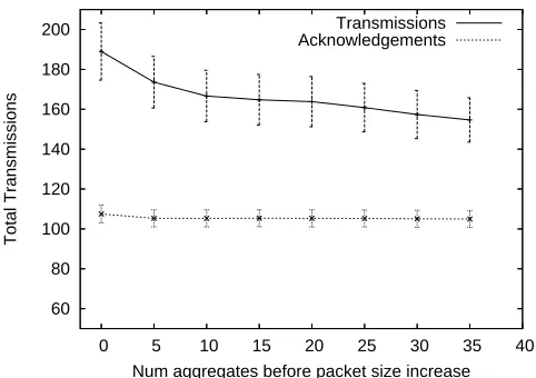
Fig. 7. Effect of increasing packet size on number of transmissions needed

of retransmissions necessary. Naturally as the BER estimation error increases to larger values the control methodology used fails to meet the required target.

F. Experiment 3

Experiment 3 examines the effects of increasing packet size on the total amount of transmissions needed to deliver all 99 messages in a gathering round. The purpose of this experiment is to examine the cost of implementing the scheme described for a number of aggregation scenarios (packet stuffing, in-network processing and pre-processing, etc.). An allowance is made for the number of aggregates that can be contained in a fixed size packet of 160 bits (this can be seen on the x-axis). When this is exceeded the length of the packet is incremented by 16 bits per extra aggregate. As before a constant BER of

0.002is used and the desired reliability,R, is 0.7.

While the number of retransmissions needed to send an aggregate packet successfully can grow quite large this is off set by the reduction of messages due to aggregation. However it must be pointed out that as packet size grows the energy need to transmit and receive a single packet also grows and therefore the graph presented does not represent the actual energy cost to the network. Nevertheless a significant energy saving is likely even in the worst case scenario where no data are aggregated without increasing packet length (leftmost part of x-axis in figure 7). Consider that without aggregation and not including retransmissions (assuming a perfect link) a minimum of 615 transmissions and acknowledgements would be needed to transport all 99 sensor data to the sink.

VIII. CONCLUSION& FUTUREWORK

The results clearly show that aggregation does not affect the probable amount of data delivered but has an adverse effect on the fluctuations about this value. These fluctuations lead to unstable application level quality and are undesirable. Having quantified the effects of aggregation a methodology is presented to determine the correct end-to-end reliability level necessary to control these effects by selecting and

implementing the correct hop-by-hop reliability, dynamically in-network, for any given aggregate size. It has been shown that this method can be used effectively to meet application specified targets.

Future work shall consider the distribution of packet losses and how these are affected by aggregation. In addition the applicability of the methods discussed in this paper will be examined with non-periodic poisson generated traffic. An examination of the current scheme and its effects on contention based MAC protocols for varying traffic conditions shall be undertaken.

IX. ACKNOWLEDGEMENTS

The support of the Informatics Commercialisation Initia-tive of Enterprise Ireland is gratefully acknowledged. Mr. O’Donovan is supported by Microsoft Research through its European PhD Scholarship Programme and the EMBARK Ini-tiative of the Irish Research Council for Science, Engineering and Technology.

REFERENCES

[1] J. Gehrke, Y. Yao. Query Processing for Sensor Networks. IEEE Pervasive Computing 2004, vol 3, number 1, pages 46-55.

[2] P. Bonnet, J. Gehrke, T. Mayr, P. Seshadri. Query Processing in a Device Database System. Tech. Report, number 99-1775, Cornell University, Ithaca, NY, USA, 1999.

[3] S. Madden, M. J. Franklin, J. M. Hellerstein, W. Hong. TAG: a Tiny AGgregation Service for Ad-Hoc Sensor Networks. Proc. of the 5th Annual Symposium on Operating Systems Design and Implementation, 2002.

[4] J. Beaver, M. A. Sharaf, A. Labrinidis, Panos K. Chrysanthis. Power-Aware In-Network Query Processing for Sensor Data. Proc. of the 2nd Hellenic Data Management Symposium, 2003.

[5] F. Stann and J. Heidemann. RMST: Reliable Data Transport in Sensor Networks. Proceedings of the 1st IEEE International Workshop on Sensor Net Protocols and Applications, 2003.

[6] S. Mukhopadhyay, D. Panigrahi and S. Dey. Data Aware, Low Cost Error Correction for Wireless Sensor Networks. Proc. of IEEE Wireless Communications and Networking Conference, 2004.

[7] S. Bhatnagar, B. Deb and B. Nath. Service Differentiation in Sensor Net-works. Proc. of the 4th International Symposium on Wireless Personal Multimedia Communications, 2001.

[8] B. Deb, S. Bhatnagar, B. Nath. Information assurance in sensor net-works. Proc. of the 2nd ACM International Conference on Wireless Sensor Networks and Applications, 2003.

[9] B. Deb, S. Bhatnagar and B. Nath. ReInForM: Reliable Information Forwarding using Multiple Paths in Sensor Networks. Proc. of the 28th Annual IEEE Conference on Local Computer Networks, 2003. [10] A. Kopke, H. Karl and M. Lobbers. Using energy where it counts:

Protecting important messages in the link layer. Proc. of the IEEE European Workshop on Wireless Sensor Network, 2005.

[11] J. Benson, U. Roedig, A. Barosso, C. Sreenan. On the Effects of Aggregation on Reliability in Sensor Networks. Proceedings of the 65th Vehicular Technology Conference, 2007.

[12] T. He, L. Gu, L. Luo, T. Yan, J. Stankovic, T. Abdelzaher, S. Son, An Overview of Data Aggregation Architecture for Real-Time Tracking with Sensor Networks. Workshop on Parallel and Distributed Real-Time Systems, 2006.

[13] M. Enachescu, A. Goel, R. Govindan, R. Motwani, Scale-Free Aggrega-tion in Sensor Networks, Theoretical Computer Science: Special Issue on Algorithmic Aspects of Wireless Sensor Networks, Vol. 344, pp. 15-29, 2005.

[14] N. Shrivastava, C. Buragohain, D. Agrawal, S. Suri: Medians and beyond: new aggregation techniques for sensor networks. Proceedings of SenSys 2004.