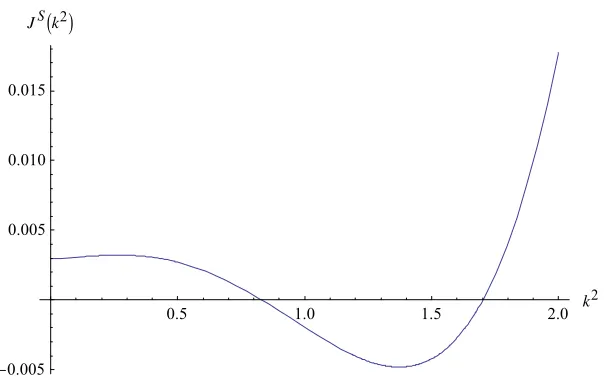
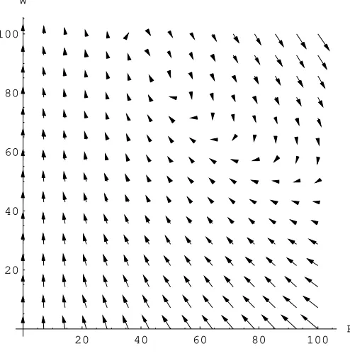
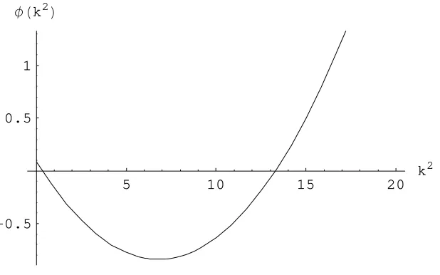
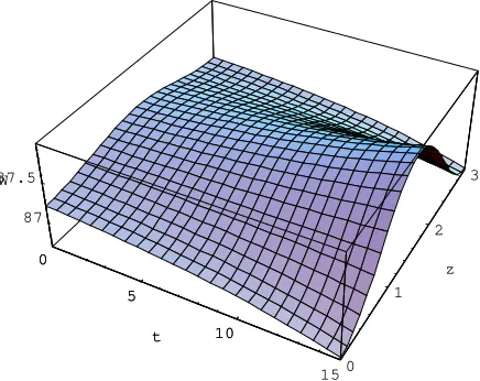
Pattern Formation, Spatial Externalities and Regulation in Coupled Economic Ecological Systems

Collected RNA-Seq data on reference Sorghum bicolor gene models was examined under the RP methodology, effectively creating individual compilations of active expression

Reduce heat to medium & cook 20-25 minutes or until potatoes are fork-tender & chili has thickened, stirring occasionally.. 2,000 calories a day is used for general

Aiming at the pose regression problem, a deep neural network architecture for RGB-D images is introduced, a training method by stages for the dual-stream CNN is presented,

According to this question, we distinguish between three different types of cooperation agreements in order to analyse to what extent the experience in cooperating with one type

Reducing the impact of maladaptive emotional memories on behaviour could be achieved by two retrieval-dependent manipulations that engage separate mnemonic processes:

 Activity patterns: mode share, travel, trip, fuel content, fuel consumption, travel patterns from transportation inventories.  Great way to get comprehensive, often official

Non-problem drinking at the 12-month follow-up was more likely in clients with a higher life satisfaction, those with lower alcohol use, those aiming for alcohol abstinence, and

In this study, we predict that three proactive career behaviours (individual career management, networking and proficiency in computer skills) will influence objective and subjective