A particle filter for freeway traffic estimation

A Particle Filter for Freeway Traffic Estimation

Lyudmila Mihaylova

Ren´e Boel

Department of Electrical and Electronic

SYSTeMS, Universiteit Gent

Engineering, University of Bristol, Merchant

Technologiepark - Zwijnaarde 914

Venturers Building, Woodland Road, UK

B-9052 Gent, Belgium

[email protected]

[email protected]

Abstract— This paper considers the traffic flow estimation problem for the purposes of on-line traffic prediction, mode detection and ramp-metering control. The solution to the estimation problem is given within the Bayesian recursive framework. A particle filter (PF) is developed based on a free-way traffic model with aggregated states and an observation model with aggregated variables. The freeway is considered as a network of components, each component representing a different section of the traffic network. The freeway traffic is modelled as a stochastic hybrid system, i.e. each traffic section possesses continuous and discrete states, interacting with states of neighbor sections. The state update step in the recursive Bayesian estimator is performed through sending and receiving functions describing propagation of perturba-tions from upstream to downstream, and from downstream to upstream sections. Measurements are received only on boundaries between some sections and averaged within regular or irregular time intervals. A particle filter is developed with measurement updates each time when a new measurement becomes available, and with possibly many state updates in between consecutive measurement updates. It provides an ap-proximate but scalable solution to the difficult state estimation and prediction problem with limited, noisy observations. The filter performance is validated and evaluated by Monte Carlo simulation.

Keywords– Monte Carlo methods, Bayesian estimation, particle filters, macroscopic traffic models, stochastic hybrid systems

I. MOTIVATION

Traffic state estimation is an important part of an on-line road traffic management system. The highly nonlinear behavior of the traffic [10], with many complex interactions between vehicles, and the computational complexity due to the large size of the state space makes this problem challenging. The macroscopic

models [10] representing theaveragetraffic behavior in terms of aggregated variables (flow, density and speed at different locations) are the most suitable models for on-line implementations. Many of the proposed solutions for estimation of aggregated traffic variables are based on Extended Kalman filtering applied to such macroscopic models [26], [8], [20]. In [26] an Extended Kalman filter (EKF) is proposed (and validated by simulation) to estimate the unknown parameters and states of a stochastic version of METANET, a well-known macroscopic model [19]. In [8] an EKF is designed for estimating the number of vehicles for two roadway sections in tandem. These estimators, [26], [8], and [20] have all the advantages and disadvantages of the EKF technique: computationally cheap, but relying on a linearization of the state and measurement models which can cause filter divergence.

A framework allowing to cope with non-linear models with uncertainties of different kinds, suitable to the traffic estimation, is

the recursive Bayesian framework [22]. According to the Bayesian theory all information about the states of interest can be obtained from the posterior state distribution. The Bayesian estimation prob-lem is not analytically solvable in general, except for some special cases. Different approximate approaches have been proposed, such as Extended Kalman Filters [22], Interactive Multiple Model Fil-ters [2]. Most of them assume Gaussian distribution of the noises and are based on linearization of the state and observation models. A powerful and scalable approximate approach has recently been developed. It computes the posterior density function of the state by an empirical histogram obtained from samples generated by a Monte Carlo simulation. It is known under different names:

particle filters [7], bootstrap method [9] or condensation algo-rithm [11]. Several implementations have been investigated [1], [7], [9], [15], [24], [25]. The Monte Carlo simulation technique has been applied in areas such as robotics navigation [23], target tracking [1], [7], [3], [16], computer vision [11], [12].

In the present paper we develop a particle filter for freeway traffic flow estimation. Particle filters (PFs) are appropriate for traffic state estimation because they can cope with large, and highly nonlinear models as well as non-Gaussian signals. The structure of the particle filter corresponds closely to compositional modelling, and it allows a parallelization for different sections of the road, thus allowing a reduction in the computational time.

In [21] a solution to highway traffic estimation is proposed using a sequential Monte Carlo algorithm, based on first-order traffic models (only dynamics of the traffic density is modelled), distinguishing between the free-flow mode and the congestion mode. The traffic mode is estimated via a Monte Carlo technique, the so called mixture Kalman filter [5] which is applied for recursively estimating the traffic density. In contrast to [21], the traffic in the present paper is described by a second-order model, and we develop a filter that estimates both traffic density and speed.

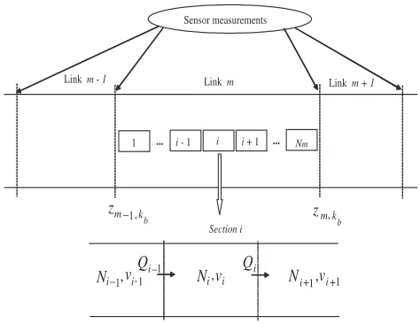
The particle filter presented in Section IV uses aggregated traffic and observation models. The state model is a recently developed compositional model [4] for freeway traffic. Sending and receiving functions describe respectively the downstream and upstream propagation of perturbations. The freeway is considered as a network of components (Fig. 1), each component representing a different section of the traffic network. Several sections form a link. Sensors are available only at some boundaries between sections. Measurements are averaged over regular or irregular time intervals before being transmitted to the estimation agent. Within the estimation agent an update of the conditional distribution of the traffic density and speed estimate is performed using Monte Carlo simulation (for all sections concurrently and possibly via parallel processing). Whenever a new measurement is received a Bayesian update of this conditional distribution is evaluated via the PF. The PF can easily be extended to models where for the very important sections a detailed model is used, while for other sections a more aggregate, coarse model is employed.

43rd IEEE Conference on Decision and Control December 14-17, 2004

Atlantis, Paradise Island, Bahamas

b k m

z

,

b k m

z

−1,

1 − i

Q

Section i

i

Q

1

1, -− i i

v

N

N

i,

v

i

N

i+1,

v

i+1

Sensor measurements

1 ... i- 1 i i+ 1 ... Nm

[image:2.612.60.297.74.257.2]

Linkm - 1 Linkm Linkm + 1

Fig. 1. Freeway links, sections and measurement points. Qi is

the average number of vehicles at the boundary between sections i and i+ 1, Ni and vi are respectively the average number of vehicles and speed within sectioni.

The outline of the paper is as follows. Section II contains the problem formulation. Section III presents the traffic and observation models. The models we are using are stochastic and macroscopic. A particle filter for traffic state estimation is designed in Section IV and its performance evaluation is presented in Section V. Finally, conclusions and ongoing research issues are highlighted in the last section.

II. PROBLEM FORMULATION

The aim of Bayesian estimation is to evaluate the posterior probability density function(PDF)p(xk|Zk)of the state vectorxk at timetkgiven a setZkof sensor measurements available at time

tk.The conditional PDF of the state vector is represented in a PF implementation by the histogram corresponding to a collection of random samples, obtained by Monte Carlo simulation, executed according to the assumed model. In this paper we propose an algorithm forestimationof the traffic state vectorxk,at discrete time instantst1, t2, . . . , tkb, . . . ,using all the past information that

was transmitted from sensors to the estimation agent prior to time tk.The same method can be used forpredictionof a future state, i.e. E(xk+1|Zk). E(.) denotes the expectation operator,E(.|.) denotes the conditional expectation operator, and (.)T the matrix transpose, respectively.

The traffic flow is modelled as astochastic hybridsystem, with continuous and discrete (modal) states, interacting with states from neighboring sections. The global state of link m at time tk is described by the vector xk = (xT1,k, xT2,k, . . . , xTnm,k)T, xk ∈

Rnx_{, containing local state vectorsx}

i,k = (Ni,k, vi,k)T ofnm sections forming this link.Ni,k is the number of vehicles counted in sectioni, andvi,k is their averagespeed. The state vectorxkis sampled at possiblyasynchronouspoints in timet1< t2< . . . <

tk< . . . .The evolution from one sample time to the next sample time is described by the update equation

xk+1=f(xk,Pk, Qink , vink , Qoutk , voutk , ηk). (1)

Pk denotes the vector of all time-varying parameters, such as road conditions, or number of available lanes; Qin_k counts the number of vehicles entering section1during thek-th time interval

[tk, tk+1)whilevin

k is the average speed of these vehicles.Qoutk specifies the possible outflow, at speedvout

k from sectionnm. ηk is a disturbance vector, reflecting random fluctuations in the traffic states, and modelling errors. The traffic mode in sectioniin this interval can make sudden transitions between different modes with rates which depend on the state vectorsxi−1,k,xi,k,xi+1,k.Note that the variables in eq. (1) are related to variables which are not indicated on Fig. 1 (input and output flows at section boundaries 0 andNm and time-varying parameters).

Sensors (magnetic loops or video cameras) are located at some boundaries between some sections j ∈ J ⊂ {1, . . . , nm} in linkm. Noisy measurements of the average number of vehicles Qi,kb, cars and trucks crossing the boundary between section j

and sectionj+ 1 during the time interval [tkb, tkb+1) together with noisy measurements of mean speed of these vehicles are collected and used by the filter. The intervals[tkb, tkb+1)can be non-equidistant points in timeand are typically longer than the intervals[tk, tk+1)between successive state update steps. Within

the intervals[tkb, tkb+1)several state update steps are required.

Given the observation equation

zkb+1=h[xs, s∈[tkb, tkb+1), ξkb+1], (2)

as well as the distributionp(x0)of the initial state vectorx0, and of the noisesηk,ξkb, the traffic estimation problem can be solved

by a particle filter having the structure presented in Section IV. The time indices in equation (2) outline that the data are coming in some intervals [tkb, tkb+1), at regular or irregular instants. The model can deal with missing data due to sensor failures or due to other reasons, by defining a functionh that takes the value “no data” with some probability. Refined models using data classified per category (cars and trucks) and per lane can also be accommodated in our PF filter.

III. TRAFFIC AND OBSERVATION MODELS

A. Traffic model

The traffic dynamics is modelled in this paper using sending and receiving functions to reflect the complex traffic behavior which incorporatesforward and backward propagation of traffic perturbations. Sending and receiving functions were first proposed by Daganzo in [6] where piecewise affine representations of these sending and receiving functions are used. In [4] a model is introduced that also represents the evolution of the average speed in each section, that comprisesspeed dependentsending and receiving functions. We briefly describe this model below since it takes part in the state update step of the particle filter developed in Section IV.

The number of vehicles, Ni,k, [veh], present in a freeway section i(with lengthLi, [km], and with i,k lanes) at sample timetkis related to thedensityρi,k(number of vehicles per length unit,[veh/km/lane]) via

Ni,k=ρi,kLii,k, i= 1,2, . . . nm. (3)

The evolution ofNi,kis governed by the conservation of vehicles:

Ni,k+1=Ni,k+Qi−1,k−Qi,k, (4)

whereQi,kis thenumber of vehicles,[veh],crossing the boundary

i(Fig. 1), leaving sectioniand entering sectioni+ 1,during the interval[tk, tk+1).Qi,k is the minimum

Qi,k=min(Si,k, Ri,k+1), (5)

among the values computed from asending function

Si,k=max{Ni,k

vi,k∆tk

Li +

ηSi,k, Ni,k

vout,min∆tk

Li }

and a receiving function

Ri,k+1=Nimax+1,k+Qi+1,k−Ni+1,k, (7)

where

N_imax_+1,k = (Li+1i+1,k)/(A+vi+1,ktd). (8)

The sending function Si,k is a random variable expressing how many among theNi,kvehicles in sectioniattk are at a distance less thanvi,k∆tkfrom the boundary between sectionsiandi+1, where ∆tk = tk+1 −tk is the sampling interval. When the density is low (corresponding to free-flow mode of traffic, i.e. when Ni,k ≤ ρcritLi,ki,k; ρcrit denotes the critical density) the interaction between vehicles will be negligible and their location will be uniformly distributed over Li. Si,k is then a binomial random variable with Ni,k drawings, with probability of success(vi,k∆tk)/Li. If the traffic is congested, vehicles will be approximately equidistantly spaced and the noise is small (relative toSi,k)and approximately Gaussian (by the central limit theorem). This formula for Si,k does not take into account what happens when a severe traffic jam causes stopped traffic at time tk in sectioni.The speed then drops to0and no vehicle would ever leave sectioniafter timetk,even if the downstream section was empty. Hence, we have to impose a minimum outflow speed vout,min with which vehicles attempt to leave section i. This minimal outflow speed can only be realized if the downstream section is not too congested, which effect is taken into account by the receiving function. This outflow speedvout,minis chosen so thatρjamvout,mini,k equals the empirically observed outflow from a traffic jam into an empty downstream section, a value that is typically significantly smaller than the maximum flow.

Each vehicle must be detected at least once in each section, during the time interval [tk, tk+1) so that this definition of the sending function to make sense. This can be expressed mathe-matically as vi,max∆tk < Li, which is similar to the stability condition in classical numerical solutions of partial differential equation models of traffic.

Thereceiving function(7) expresses the maximum number of vehicles that are allowed to enter section i+ 1 at the next time instantk+ 1. In this formulaN_imax+1,k characterizes themaximum

number of vehiclesthat can simultaneously be present in section i + 1 at sample time tk. It is given by the available space

Li+1i+1,k in sectioni,divided by the speed-dependent “virtual length” of vehicles. This virtual length of vehicles is the average space needed by a vehicle: its average lengthAplus the distance travelled during a minimum time distancetdbetween two vehicles (necessary to allow safe driving). vi,k is the average speed of vehicles inside section iat timetk.In order to prevent possible negative values ofRi,k+1(7) when abrupt changes happen in the

capacity of a section (e.g. provoked by changes in the number of lanes due to an incident), the model imposes

Ni+1,k=Nimax+1,k, if Nimax+1,k< Ni+1,k. (9)

The sending function causes downstream propagation of pertur-bations in the traffic density. It can be recursively calculated from left to right. The receiving function on the other hand corresponds to upstream propagation of traffic density perturbations, and it must be recursively calculated from right to the left. Evidently, updating the number of vehicles in thenmdifferent sections from its value at timetkto its value at timetk+1requires the solution

of a system withnmnonlinear algebraic equations(4)-(8). In our algorithm we iteratively solve this set of equations as follows. The sending function is calculated at first by forward recursion, and we substitute Qi,k = Si,k in (4). With this “first guess” of the number of vehicles in section iat timetk+1 a first guess of the

density and the speed at time tk+1 are calculated. After that a

first guess of the receiving function can be computed, recursively

from sectionNmdown to section1.This means that the number of vehicles leaving sectionimust be smaller than or equal to the number of vehicles that the neighbor section can receive. In the algorithm the number of vehicles passing boundaryiis calculated by the rule [4]:

if Ri,k+1 < Si,k, then Qi,k=Ri,k+1,

∆i,k=Si,k−Ri,k+1, Ni,k+1=Ni,k+1−∆i,k. (10)

This iteration is repeated until no further changes in the flowsQi,k are made. In a finite number of iterations this leads to the correct numberQi,k of vehicles which actually are succeeding to cross the boundary, whereas ∆_i,k = Si,k−Ri,k+1 is the number of

vehicles which are forced to remain in sectioniby slowing down. The speedvi,k+1is updated according to the rule:

v_i,kinterm+1 =

⎧ ⎪ ⎪ ⎪ ⎨ ⎪ ⎪ ⎪ ⎩

[vi−1,kQi−1,k+vi,k(Ni,k−Qi,k)]/Ni,k+1,

forNi,k+1= 0,

vf ree, otherwise,

(11)

ρantic_i,k+1=αρi,k+1+ (1−α)ρi+1,k+1, (12)

vi,k+1=βvintermi,k+1 + (1−β)ve(ρantici,k+1) +ηvi,k, (13)

where v_i,kinterm₊₁ is the intermediate speed taking convection into account. It expresses the speed update if all vehicles would maintain their speed forever: drivers can not change their speed instantaneously due to inertia. ρantic_i,k+1 is the anticipated traffic density which drivers see at some distance in front of their vehicles, and ρi,k+1 is computed from (3) after Ni,k+1, i =

1, . . . , nmhas been evaluated. The coefficientα∈(0,1]weighs how far ahead the drivers are looking in their anticipation (largest lookahead for α close to 1). The function ve(ρ) expresses the average speed corresponding to densityρ.This equilibrium speed can be computed according to the empirical equation given in [14], [19] but for our model we find that simpler expressions are sufficient. When the density is below the critical density ρcrit we assume that the desired speed is equal to the free flow speedvf ree.In congested regime the average speed drops affinely from vf ree at ρcrit to 0 at ρjam. The coefficient β ∈ (0,1] tunes the model by weighing how aggressively drivers adjust their speed to changing traffic conditions. The noiseηvi,k reflects the unpredictable behavior of the drivers and also modelling errors. It is assumed in our simulations to have a Gaussian distribution.

Given the initial vectorx0= (N1,0, v1,0, . . . , Nnm,0, vnm,0)T,

and the boundary variables (the sending functions S0,k at the upstream boundary of section 1, and the receiving functions Rnm+1,k at the downstream boundary of section nm) one can now evaluate the random evolution of the statexkof the freeway, using (4) and (13) as state update equations (1).

B. Observation equations

The following observation equations are derived in agreement with (2)

zj,kb+1(1) = ¯Qj,kb+1+ξQj,kb+1, (14)

zj,kb+1(2) = ¯vj,kb+1+ξvj,kb+1. (15)

zj,kb+1(1)is the measured averaged number of vehicles crossing

the boundary between sectionsjandj+1during the time interval

∆tb = [tkb, tkb+1), namely Q¯j,kb+1 = ∆1tb

k=tb+1

that this average speed weighs the faster vehicles more heavily than the slower vehicles, since faster vehicles cross boundaries more frequently. The noise term ξQj can have a complicated

probability distribution (e.g. Poisson type, when errors due to missed vehicles and false counted vehicles are accounted for).

IV. PARTICLE FILTER FOR FREEWAY TRAFFIC

Within the Bayesian framework, the conditional density p(xk|Zk−1)is recursively updated according to

p(xk+1|Zk) =

Rnxp(xk+1|xk)p(xk|Z

k_)dx

k, (16)

p(xk|Zk) =

p(zk|xk)p(xk|Zk−1)

p(zk|Zk−1)

, (17)

wherep(zk|Zk−1)is a normalizing constant. The recursive update ofp(xk|Zk) is proportional to

p(xk|Zk)∝p(zk|xk)p(xk|Zk−1). (18)

Usually, there is no simple analytical expression for propagating p(xk|Zk)through (18).

The particle filter technique [7] provides an approximate so-lution to this discrete-time recursive updating of the posterior

probability density function p(xk|Zk) of the state given mea-surementszj,kb+1(1), zj,kb+1(2)forj∈J⊂ {1, . . . , nm}. The state update and the measurement update steps use respectively the conditional density functions p(xk+1|xk) andp(Zk|xk) that are defined uniquely by the model described in sectionIII.The particle filter approximates p(xk|Zk)by the empirical histogram corresponding to a collection ofMparticles (samples){x(_kl)}M_l=1. Each particle has an assigned relative weight, w_k(l), such that the sum of all weights is unity. The weight and the value of each particle characterize (an approximation to) the conditional density function of the state xk. After the arrival of a new observationzkb, the particle filter updates the value of the particles

location and their weights according to Bayes’ rule. The cloud of particles evolves with time and depending on the observations, so that the particles represent with sufficient accuracy the true conditional density of the state. Note that we treat a problem that is slightly more complicated than in the previously developed particle filters [7]. The sensor information updates the state distribution usually assuming that the observation at time tk is a noisy function of the state at timetk, while in the traffic problem the observation at time tk depends on the values of the state at all the times{tkb−1, . . . , tkb−1, tkb}through an averaging operation.

This extension can easily be incorporated in the PF algorithm. During the interval[tkb, tkb+1), between two consecutive mea-surement updates, traffic state prediction is performed through the traffic models (4), (5), (6) and (7) for the nm sections. The likelihood function p(zk|xk)is calculated from (14)-(15) by the predicted states at each of the time instants tk ∈ [tkb, tkb+1), and the known measurement noise densitypξi,k(ξi). The cloud of weighted particles, drawn from the posterior conditional probabil-ity distribution, is used to map integrals to discrete sums (since the histogram is piecewise constant): p(xk|Zk) is approximated by

ˆ

p(xk|Zk)≈ M

l=1 ˜

w_k(l)δ(xk−x(kl)), (19)

where δ is the delta-Dirac function andw˜_k(l) are the normalized importance weights of the posterior conditional probability density function (PDF). New weights are calculated putting more weight on particles that are important according to

the posterior probability density function (19). The random samples{x(_kl), l= 1,2, . . . , M} are drawn fromp(xk|Zk). It is often impossible to sample from the posterior density function p(xk|Zk). However, this difficulty is circumvented by making use of the importance sampling from a knownproposal distribution π(xk|Zk). In implementing particle filters, the choice of the proposal distribution is of crucial importance. The transition prior is the most popular choice of the proposal distribution [25]: π(xk|Zk) = p(xk|xk−1), which in the traffic problem is given by the traffic state model.

The implementation of the particle filter is described below:

1) Initialization:k= 0

* For l = 1, . . . , M, generate samples {x(₀l)} from the initial distributionp(x0).

2) Fork= 1,2, . . . , km, . . ., * Prediction step :

For l = 1, . . . , M, sample x(_kl) ∼ p(xk|x(kl−)1, Zk)

according to (3)-(13) for sections situated between two subsequent boundaries where measurements arrive.

* Evaluate importance weights (measurement processing step), only for k = kb, on the boundaries between the sections where measurements are available. On the receipt of a new measurement, compute the weights

w_k(l)=w_k(l₋)₁p(zk|x(kl))

and normalize, i.e. wˆ(_kl) = w_k(l)/M_l=1w(_kl). The observation equations (14), (15) describe the likelihood p(zk|x(kl)) of the observations. Note that the form of equations (14) and (15) reduces the computational costs, because the predicted observations will actually coincide with the predicted number of vehicles on the boundaries and predicted speeds, obtained from the prediction step.

* Selection step (resampling) only fork=kb:

Multiply/ Suppress samplesx(_kl) with high/ low importance weights wˆ(_kl), in order to obtain M random samples approximately distributed according to p(xk|Zk). The residual resampling algorithm described in [17], [25] is applied. This is a two step process making use of sampling-importance-resampling scheme.

* Fori= 1, . . . , M, setw_k(l)= ˆw_k(l)= 1/M.

3) Output: The output of the algorithm is a collection of sam-ples, from which the approximate posterior distribution is computed according to (19). The posterior meanE[xk|Zk] and the associated covarianceV[xk|Zk]are approximately computed using the collection of samples (particles), namely

ˆ

xk=E[xk|Zk] = _M1 _M

l=1x(kl),

V[xk|Zk] = _M1_{−1 M}

l=1(x(kl)−ˆxk)(x(kl)−xˆk)T.

4) Increasek and return to step 2.

freeway network for the purposes of on-line traffic management.

V. FILTER PERFORMANCE EVALUATION

The particle filter performance is evaluated by Monte Carlo simulation over independent Monte Carlo runs with different collections of data, different initial state conditions and different boundary conditions. The data are generated by using a stochastic version of METANET model [14], [19], after adding Gaussian noises to the speed and density equations. The measurements are supplied to the filter every minute, similarly to a possible update with real data, whereas the state prediction is performed also in the intermediate time instants. We are estimating the states of all sections between two sensor locations as one augmented state vector, composed by mutually connected components.Root-Mean Squared Errors (RMSEs) [2] (ˆxi) = [1_r

_r

i=1(εi,k)T(εi,k)]1/2, for relative state errors, εi,k = (xi,k −xˆi,k)/xi,k, e.g., w.r.t. density, speed and flow (the same state variables such as in METANET) are used to evaluate the filter performance.

Investigations with simulated data

The link considered consists of four sections, with mea-surements received only at the boundaries of the first and fourth section. Hence, the augmented state vector is xk =

(xT_1,k, xT_2,k, xT_3,k, xT_4,k)T, i.e.i= 1,2,3,4, and the measurement vector zkb = (z1T,kb, z4T,kb)T. The boundary conditions (inflow

and speed at entrance boundary and density and speed in section nm+1) are assumed known, not estimated. In order to see the

often used in practice flow-density and speed-flow diagrams from the states, the plots are given in terms of flows, densities, speeds. The initial section states are randomly generated from the true states using Gaussian distribution, i.e. x0 ∼ N[x0, P0], where x0 contains the exact initial state vector and P0 is the initial state covariance matrix. The size of the sample set is M = 500 particles.

1 2 3 4

0 0.1 0.2 RMSE : ρ1 RELATIVE RMSEs

1 2 3 4

0 0.05 0.1

RMSE : v

1

1 2 3 4

0 0.02 0.04

RMSE : q

1

1 2 3 4

0 0.1 0.2

RMSE :

ρ2

1 2 3 4

0 0.05 0.1

RMSE : v

2

1 2 3 4

0 0.02 0.04

RMSE : q

2

1 2 3 4

0 0.1 0.2

RMSE :

ρ3

1 2 3 4

0 0.05 0.1

RMSE : v

3

1 2 3 4

0 0.02 0.04

RMSE : q

3

1 2 3 4

0 0.1 0.2

RMSE :

ρ4

1 2 3 4

0 0.05 0.1

RMSE : v

4

1 2 3 4

0 0.02 0.04

RMSE : q

4

[image:5.612.319.548.73.282.2]

Time, [h]

Fig. 2. Relative root-mean square errors of the density (for all lanes), speed and flow of the four sections

The parameters of the state model are chosen as follows: ρi,crit= 32.5 [veh/km/lane],∆t= 10 [sec],Li= 0.5 [km],

i= 1,2,3,4,α= 0.9,β= 0.6,A= 0.010 [km],am= 1.867.

1 2 3 4

−2 −1 0 ME : ρ1 RELATIVE MEs

1 2 3 4

−1 −0.5 0 0.5

ME : v

1

1 2 3 4

−0.2 0 0.2 0.4

ME : q

1

1 2 3 4

−2 −1 0

ME :

ρ2

1 2 3 4

−1 −0.5 0 0.5

ME : v

2

1 2 3 4

−0.2 0 0.2 0.4

ME : q

2

1 2 3 4

−2 −1 0

ME :

ρ3

1 2 3 4

−1 −0.5 0 0.5

ME : v

3

1 2 3 4

−0.2 0 0.2 0.4

ME : q

3

1 2 3 4

−2 −1 0

ME :

ρ4

1 2 3 4

−1 −0.5 0 0.5

ME : v

4

1 2 3 4

−0.2 0 0.2 0.4

ME : q

4

[image:5.612.314.554.333.546.2]

Time, [h]

Fig. 3. Relative MEs of the density (for all lanes), speed and flow of the four sections

0 100 200 300

0 2000 4000 6000 8000 10000 Flow(density) diagram Density, [veh/km] Flow, [veh/h]

0 2000 4000 6000 8000 10000

0 20 40 60 80 100 120 140 Flow, [veh/h] Speed, [km/h] Flow(speed) diagram

1 2 3 4

0 2000 4000 6000 8000 Flow, veh/h] Time, [h]

1 2 3 4

0 50 100 150 Speed, [km/h] Time, [h] 1 2 3 4 4 3 2 1

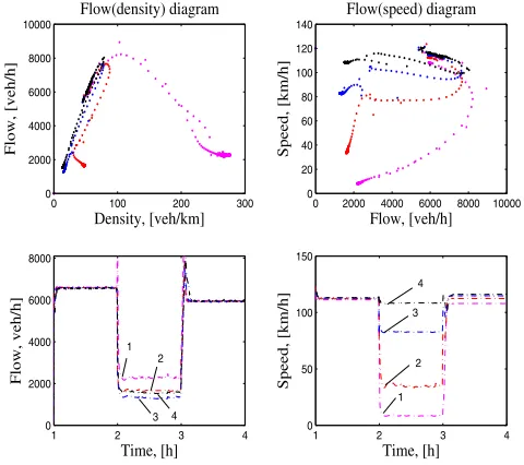
Fig. 4. Flow-density, flow-speed diagrams, evolution of the flow and of the speed in time plotted from the estimated states

We assume that the free flow speed vf ree is 130 [km/h], the minimum outflow speed isvout,min= 3 [km/h].

In the initial investigation we assumed that the number of lanes is known (but this could be estimated recursively). The simulations assumei,k = 3 always except for a reduction to i,k = 1 in lanesi= 2,3 fortk between2 [h]and 3 [h]. The model error and the measurement noise are assumed to be Gaussian, where cov(ηvi) = 0.52[km/h]2, the covariance of the sending function

is non-stationary:cov(ηSi,k) = (0.025Ni,kvi,k∆tk/Li)2 [veh]2, andVξi=diag{202 [veh/h]2, 22[km/h]2.

The filter performance is evaluated forr = 100 independent Monte Carlo runs. Relative Root-mean square errors (RMSEs)

[image:5.612.64.294.458.665.2]

and relative mean errors (MEs) in Fig. 3. Fig. 4 contains the flow-density, speed-flow diagrams, and shows the evolution of the average traffic flow and of the average speed in time. All figures are plotted from the estimated states. According to these results the particle filter can accurately estimate the traffic states except for a very brief increase in error during the fast transients. The flow-density diagram, based on the estimates has a bell-shaped form in good agreement with the well known fundamental diagram [18]. The evolution of the estimated speed in time shows that the traffic in section 1 is characterized with a decreased speed during the period with reduced number of lanes in sections 2 and 3 (between

2 [h]and3 [h]. So far experiments have been performed with one link consisting of four sections. The application of the particle filter to many links of the freeway is straightforward.

Probabilistic traffic mode detection is currently investigated based on multiple modelling of different traffic modes, also the formulation of criteria for on-line modes detection and the transitions between them. Typical traffic modes can be represented by few models which together with the observations can provide likelihood ratios. Likelihoods are then bringing information about the correct model/ mode. One of the difficulties is the appropriate classification of the traffic modes. Multiple-model particle filters can be used for change and mode detection as well. To each mode a separate model is assigned and based on the measurements the wrong models will have high innovation processes, respectively small likelihoods which means that they will be less probable and hence rejected.

VI. CONCLUSIONS

The freeway traffic flow estimation is formulated within a Bayesian recursive framework. A particle filter is developed using traffic and observation models with aggregated variables. The traffic state is modelled as a hybrid stochastic system, i.e. the traffic section possesses continuous and discrete states, interacting with states from neighbor sections. The filter performance is investigated and validated by simulated data. The designed particle filter gave very encouraging performance. Currently investigations are conducted with real traffic data from a Belgian freeway. The estimation approach presented is straightforward, general, and applicable to both freeways and urban networks, with different topologies, with any number of sensors, regularly or irregularly received data in space and in time. It is suitable for distributed realization and for parallel computations. The presented approach for traffic state estimation is modular. Different traffic models can be used in different sections of the traffic network. This recursive Bayesian estimator is aimed at on-line applications for mode detection, and in different control strategies of road traffic, for instance it fits well in the model predictive control framework.

REFERENCES

[1] M. Arulampalam, S. Maskell, N. Gordon, T. Clapp, A Tu-torial on Particle Filters for Online Nonlinear/Non-Gaussian Bayesian Tracking, IEEE Trans. on Signal Proc., 2002, Vol. 50, No. 2, pp. 174-188.

[2] Y. Bar-Shalom, X. R. Li,Estimation and Tracking: Principles, Techniques, and Software, Boston MA, Artech House, 1993. [3] N. Bergman, Recursive Bayesian Estimation. Navigation and

Tracking Applications, Ph.D. thesis, Dept. of Electrical Engi-neering, Link¨oping, Sweden, 1999.

[4] R. Boel and L. Mihaylova, Modelling Freeway Networks by Hybrid Stochastic Models, Proc. of the IEEE Intelligent Vehicle Symposium, Parma, Italy, pp.182-187, 2004.

[5] R. Chen and J. Liu, Mixture Kalman filters,Journal of Royal Statistical Society B, Vol. 62, pp. 493-508, 2000.

[6] Daganzo, C., The Cell Transmission Model: A Dynamic Representation of Highway Traffic Consistent with the Hydro-dynamic Theory,Transportation Research B, Vol. 28B, No. 4, pp. 269-287, 1994.

[7] A. Doucet, N. Freitas, and N. Gordon, Eds.,Sequential Monte Carlo Methods in Practice, New York: Springer-Verlag, 2001. [8] D. Gazis, and C. Liu, Kalman Filtering Estimation of Traffic Counts for Two Network Links in Tandem, Transportation Research B, Vol. 37, No. 8, 2003, pp. 737-745.

[9] N. Gordon, D. Salmond, and A. Smith, A Novel Approach to Nonlinear / Non-Gaussian Bayesian State Estimation, IEE Proc. on Radar, and Signal Proc., Vol. 40, pp. 107-113, 1993. [10] D. Helbing, Traffic and Related Self-Driven Many-Particle Systems,Rev. of Modern Phys., Vol. 73, pp. 1067-1141, 2001. [11] M. Isard, and A. Blake, Contour Tracking by Stochastic Propagation of Conditional Density, Proc. of the European Conf. on Comp. Vis., Cambridge, UK, 1996, pp. 343-356. [12] M. Isard, and A. Blake, Condensation – Conditional Density

Propagation for Visual Tracking, International Journal of Computer Vision, Vol. 28, No. 1, 1998, pp. 5-28.

[13] Y. Kim,Online Traffic Flow Model Applying Dynamic Flow-Density Relations, Ph.D. thesis, Techn. Univ. M¨unchen, 2002. [14] A. Kotsialos, M. Papageorgiou, C. Diakaki, Y. Pavis and F. Middelham, Traffic Flow Modeling of Large-Scale Motorway Using the Macroscopic Modeling Tool METANET, IEEE Trans. on Int. Transp. Syst., Vol. 3, No. 4, pp. 282-292, 2002 [15] J. Liu, Monte Carlo Strategies in Scientific Computing,

Springer-Verlag, 2001.

[16] Special Issue on Monte Carlo Methods for Statistical Signal Processing,IEEE Trans. on Signal Proc., Vol. 50, No. 2, 2002. [17] J. Liu and R. Chen, Sequential Monte Carlo Methods for Dynamical Systems,Journal of the American Statistical Asso-ciation, Vol. 93, pp. 1032-1044, 1998.

[18] A. D. May,Traffic Flow Fundamentals, Prentice-Hall, En-glewood Cliffs, New Jersey, 1990.

[19] M. Papageorgiou, J.-M. Blosseville, Macroscopic Modelling of Traffic Flow on the Boulevard P´eriph´erique in Paris, Trans-portation Research B, Vol. 23, No. 1, pp. 29-47, 1989. [20] S. Smulders,Control of Freeway Traffic Flow, Ph.D. thesis,

Universiteit Twente, 1989, Netherlands.

[21] X. Sun, L. Mun˜oz, R. Horowitz, Highway Traffic State Esti-mation Using Improved Mixture Kalman Filters for Effective Ramp Metering Control, Proc. of 42th IEEE Conference on Decision and Control, pp. 6333–6338, 2003.

[22] A. Sage, and J. Melsa,Estimation Theory with Applications to Communications and Control, McGraw-Hill Inc., 1971. [23] S. Thrun, Particle Filters in Robotics,Proc. of the the 17th

Annual Conf. on Uncertainty in AI (UAI), 2002.

[24] R. Van der Merwe, De Freitas, N., Doucet, A., Wan, E., The Unscented Particel Filter,Advances in Neural Information Processing Systems 13, 2001.

[25] E. Wan, and R. van der Merwe, The Unscented Kalman Filter, inKalman Filtering and Neural Networks, S. Haykin, Ed., Chapter 7, pp. 221–280, Wiley Publ., 2001.

[26] Y. Wang, M. Papageorgiou, and A. Messmer, Motorway Traffic State Estimation Based on Extended Kalman Filter,

Proc. of the European Control Conf., 1-3 Sept., 2003, UK.