http://dx.doi.org/10.4236/ojs.2013.36050
Distribution of the Median in Samples from
the Laplace Distribution
*
John Lawrence
US Food and Drug Administration, Silver Spring, USA Email: [email protected]
Received October 1,2013; revised November 1, 2013; accepted November 8, 2013
Copyright © 2013 John Lawrence. This is an open access article distributed under the Creative Commons Attribution License, which permits unrestricted use, distribution, and reproduction in any medium, provided the original work is properly cited. In accordance of the Creative Commons Attribution License all Copyrights © 2013 are reserved for SCIRP and the owner of the intellectual property John Lawrence. All Copyright © 2013 are guarded by law and by SCIRP as a guardian.
ABSTRACT
The Laplace distribution is one of the oldest defined and studied distributions. In the one-parameter model (location parameter only), the sample median is the maximum likelihood estimator and is asymptotically efficient. Approxima-tions for the variance of the sample median for small to moderate sample sizes have been studied, but no exact formula has been published. In this article, we provide an exact formula for the probability density function of the median and an exact formula for the variance of the median.
Keywords: Quantile; Generalized Hypergeometric Function
1. Introduction
Laplace is credited as first discovering the Laplace dis-tribution in 1774 [1]. The discovery of the normal distri-bution, which holds a central place in many applications of statistics, predates that of the Laplace distribution. It was discovered in 1738 by de Moivre according to [2]. Gauss and Laplace were contemporaries who both made significant discoveries about the normal distribution. Keynes [3] wrote “The popularity of the normal law, with the arithmetic mean and the method of least squares as its corollaries, has been very largely due to its over-whelming advantages, in comparison with all other laws of error, for the purposes of mathematical development and manipulation... So powerful a hold indeed did the normal law obtain on the minds of statisticians, that until quite recent times only a few pioneers have seriously considered the possibility of preferring in certain circum-stances other means to the arithmetic and other laws of error to the normal. Laplace’s earlier memoir fell, there-fore, out of remembrance.” Over the past 100 years, the Laplace distribution has enjoyed the resurgence in many applications such as economics, engineering and finance [4]. The reader is also referred to this book for a history of the Laplace distribution, its important properties and
generalizations.
Let f xx
;
exp
2 x
2 denote the pro- bability density function of a one-parameter Laplace dis-tribution with variance 1. It is well known that from a sample of odd size 2n + 1 where n is any positive integer, the sample median, , is the maximum likelihood esti-mate of μ. Moreover, although the derivative does not exist at μ, the Cramer-Rao lower bound for the mean squared error of estimation of μexists and is 1 2 2
n1
. Also, we have 2 2
n1
N
0,1 which im- plies the median is an efficient estimator in the asymp-totic sense. However, is not a sufficient statistic and there are more efficient estimators for small samples, for example the average of the middle three observations can be more efficient. Finally, the sample mean is also as-ymptotically normal and asas-ymptotically the ratio of the variance of the mean to the median is 2.Previously, [5] investigated approximations to the variance of for small sample sizes. They confirmed that although the variance converges to the Cramer-Rao lower bound, it does so at a slow rate. Consequently, even if the normal approximation was valid for small sample sizes, hypothesis tests and confidence intervals would not have the correct size if the asymptotic variance was used. The former provided the bounds for the ratio of the variance to the Cramer-Rao lower bound as
fol-*The views expressed are those of the authors and not necessarily those
lows:
3 2
3 2
1
1 2 2 1 V
2 2
1
1.51 1
2 n
n
B n
n
B n ar
where
2 2 1 ! 21
π ~ 1 1 8! !2 2 1
n n
n B
n
n n n
. For example, if
499
n and the sample size were 999, the upper bound would be approximately 1.513. This suffices for their purpose, which was mainly to show that this ratio was less than 2, which in turn implies the median is a more efficient estimator than the sample mean. However, it seems like an inadequate upper bound since we know the ratio converges to 1. [6] attempted to tabulate the ap-proximate variance for , and 8. We found that in general his approximations were close to the true values (to two digits), but were not correct in two out of these five cases (see Section 3).
1, 2,3, 4 n
This paper makes two contributions. First, we find an explicit formula for the distribution of the median of a random sample from the Laplace distribution. Next, we find an exact formula for the variance of the sample dian. These contributions are important because the me-dian is the essential estimate of location for the Laplace distribution in the same way that the mean is the essential estimate of location for the normal distribution.
2. Exact Distribution of Sample Median
Without loss of generality, we will consider the case where μ = 0. The probability the median is less than x is the probability that at least n + 1 values in the sample are less than x. The distribution of the median is symmetric about 0, so it suffices to consider values of x < 0. Then, we have
def
,
2 1 2 1
2 2
1
2 1 1 1
e 1 e
2 2
n
i n
n
x x
i n
F x P x
n i
i
In the Appendix, we show by mathematical induction that the density for x < 0 is
1 2 2,
1
e 1 e
2 n
n x x
n n
f x c
where the constants are
1 2
3
Γ
2 1
2
2 1 2
πΓ 1 n
n
n
n
c n
n n
1 2
n
.
Hence, 1e 2
2
has a Beta distribution truncated on
the interval
0,1 2
.The characteristic function is 3
2 2 1
2 ; 1 ,
2 2
it n
n
t
c B n i n
1
and the moment generating function is 3
2 2 1
2 ; 1 ,
2 2
t n
n
t c B n n
1.
In both cases, the formulas involve the incomplete beta function
1 2 1 1
0
1; , 1 d
2
b a
B a b u u
u.3. Variance of the Median
The variance can be calculated exactly using the Bino-mial expansion as
0
1 2
2 2
0
1 2 2
0
3 0
1
2 e 1 e d
2 1
2 e
2
1 1
2
2 2 1
n
n x x
n
i n
n i x
n i
i n
n i
x c x
n
c x
i n c
i n i
dx
This variance also evaluates to
31
, 1, 1 , 2, 2, 2 ,
2 2
1
p q
n
F n n n n n n
c
n
where pFq is the generalized Hypergeometric function. For n1,2,3, 4, and 8, the ratios of the variance of the median to the variance of the mean (rounded to 6 digits) are 0.958333, 0.877951, 0.824767, 0.787808, and 0.708761. In comparison to the approximations listed in the bottom row of Siddiqui, these are close in all cases. In the case of n = 3, (corresponding to a sample size of N = 7 in his notation) he gives the approximate value of 0.81, but it should be 0.82 rounded to 2 digits. Also, in the case of n = 4, he gives the approximation 0.78, while it should be 0.79.
As a further example, consider the case n = 499, cor-responding to a sample size of 999. This would be a rather large dataset by most standards and one might think the asymptotic variance would be accurate. How-ever, the ratio of the actual variance to the asymptotic value is 1.05122, or about 5% larger than the Cramer- Rao lower bound. Although not very close to 1, it is sub-stantially closer than the upper bound of 1.513 provided by the Chu and Hotelling approximation (see Section 1).
to calculate the variance exactly using the formula at the beginning of this Section. One way to estimate the ratio of the true variance compared to the asymptotic variance is
0 2 1 2 2
0 1
2 2 1 2 1
1
2 1 2 1
0 2
1
2 1 2 1
2
1
2 e 1 e d
2 1
2 2 1
2 e 1 1e d
2
2 1
1
e 1 e
2
2 d
2 1
1
e 1 e
2
2 2 1
n
n x x
n
n
x x
n
n n
n
n
x x
n
n n
n
n
Z Z
n
n n
n
x c x
n
x c x
n
c
x x
x n
c E Z
Z
n
where Z is standard normal with distribution function
Φ x and density function
x . The numerator can be estimated by Monte Carlo simulation or the integral in the second to the last line can be estimated by numerical integration such as the Riemann sum1 1
1 0
Φ
2 N
i
N h
N N
.5 where h
denotes the integrand and N is a large inte-ger.It is also possible to sample values having the density
f x by using acceptance-rejection sampling. To do this, one needs a candidate distribution with density
g x such that
f x
g x
is bounded by a fixed upper
bound M. In addition, it is best if M is close to 1 since the proportion of candidate values that will be accepted is
1 M . The Laplace distribution with variance 2 is a very good candidate distribution to sample from. Note that the ratio
1
2 1 2 1
1 1 1
2
2 2 1
2
n
x x
n
n n
n
x
c e e
n
e
attains its maximum at
1
2 2
2 1
2 1log
2
n n
n
x n
n
1
and that maximum is
2 1
2 2 1 1
2e
2 1
π
1 1
2 1
n
n
n
n
c n
n M
n
n
.
4. Conjecture about the Rate of Convergence
Start with values of n that were the closest integers to
exp 3 ,exp 4 , , exp 20 .
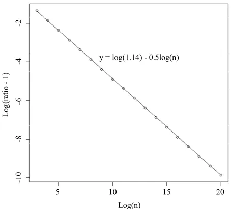
For each of those values of n, calculate the ratio given in the previous Section viathe Riemann sum described in Section 4 with N10 million. In Figure 1, we show
the values of log
n on the x-axis and log(ratio -1) on the y-axis where the ratio means the ratio of the actual variance to the asymptotic variance computed by nu-merical integration. We noticed that the points fell very close to the straight line defined by
log 1.14 0.5log
y n .
Hence, at least in this range of n, the ratio is approxi-mately 1 1.14 n. Note, the largest n here is approxi-mately 500 million, which corresponds to a sample size of about 1 billion.
This leads to a conjecture about the rate of conver-gence of the variance. In addition, from the formula near the beginning of Section 3, this is also a conjecture about the asymptotic behavior of the Hypergeometric function for large n. Specifically,
3 2 1
1
, 1, 1 , 2, 2, 2 ,
2
π 1.14
~ 1
2 2
p q
n
F n n n n n n
n
n
using Stirling’s approximation ~ 2 2
π
n n
n
c .
5. Summary and Conclusion
y = log(1.14) - 0.5log(n)
5 10 15 20
Log(n)
-10
-8
-6
-4
-2
L
og
(ra
ti
o - 1
[image:4.595.58.285.85.290.2])
Figure 1. Transformed values of ratio (actual variance of the median divided by asymptotic variance estimated by numerical integration) for different large values of n.
approach could be used to find the distribution of any other order statistic. For even sample sizes, the median is the average of the two middle observations, which makes it slightly more complicated to analyze because the joint distribution of two order statistics is needed. However, a similar approach used here may also handle the even sample size case. Furthermore, this approach could also be useful in analyzing the variance of other estimators such as the average of the middle three or middle five and observations. And it could be helpful in finding the optimal estimator for small sample sizes. This exact vari-ance may be useful in constructing approximate
confi-dence intervals or hypothesis tests. But, caution should still be used in using the normal approximation. Exact tests and confidence intervals can be constructed from the exact distribution. Lastly, in the two-parameter Laplace model, not considered here, a further adjustment may be needed in such procedures due to the estimation of the scale parameter.
REFERENCES
[1] P. S. Laplace, “Mémoire sur la Probabilité des Causes par les Évènemens,” Mémoires de Mathematique et de Phy-
sique, Presentés à l’Académie Royale des Sciences, Par Divers Savans & Lûs Dans ses Assemblées, Tome Sixième, 1774, pp. 621-656.
[2] N. L. Johnson, S. Kotz and N. Balakrishnan, “Continuous Univariate Distributions,” Vol. 1, Wiley,Hoboken, 1994. [3] J. M. Keynes, “The Principal Averages and the Laws of
Error Which Lead to Them,” Journal of the Royal Statis- tical Society, Vol. 74, No. 3, 1911, pp. 322-331.
http://dx.doi.org/10.2307/2340444
[4] S. Kotz,, T. J. Kozubowski and K. Podgorski, “The Laplace Distribution and Generalizations: A Revisit with Applications to Communications, Economics, Engineer- ing, and Finance (No. 183),” Springer, Berlin, 2001. http://dx.doi.org/10.1007/978-1-4612-0173-1
[5] J. T. Chu and & H. Hotelling, “The Moments of the Sam- ple Median,” The Annals of Mathematical Statistics, Vol. 26, No. 4, 1955, pp. 593-606.
http://dx.doi.org/10.1214/aoms/1177728419
[6] M. M. Siddiqui, “Approximations to the Moments of the Sample Median,” The Annals of Mathematical Statistics, Vol. 33, No. 1, 1962, pp. 157-168.
Appendix
First, note that for any positive integers m and i with i < m,
2 2
1
2 2
1 1
e 1 e
2 2
1 1 1
e 1 e 2 e
2 2 2
i m i
x x
i m i
2
x x i m
x
when n = 1,
2 2 2,1
1 1 1
3 e 1 e e
2 2 2
x x
F x
and
2 2 2,1 ,1 1
1 1
e 1 e
2 2
x x
f x F x c
We suppose that the formula for the density is true for some positive integer n.
Consider the random sample of size 2
n 1
3 2x
1 and recalculate the distribution function for the median of this random sample by conditioning on the number of values among the first 2n + 1 elements in the sample that are less than x. If the median of the entire sample is less than x, then there are three possible cases for such num-bers: exactly n, exactly n + 1, or at least n + 2. We have
, 1 1 2 1 2 2 2 3
1 2 1 2 2 2 3
1 2 1
1 2
2 2 2
exactly among , , and
exactly 1 of , , or
2 or more of , ,
2 1 1 1 1
e 1 e e
2 2 2
2
n n n
n n n
n
n n
x x x
n
F x P n X X x P X x X x
P n X X x P X x X
P n X X x
n n
n
x
1 2
2 2 2 2 2
1 1
2 2 2
1 1 1 1 1
e 1 e e 1 e e
1 2 2 2 2
1 or more of first 2 1 exactly 1 of first 2 1
2 1
1 e
2 2
e e
1 2
n n
x x x x x
n n
x x x n
n
P n n x
P n n x
n n
,
1 2
e x 1
n F x
The derivative is
1
2 2
2 2 2
,
2 1 e e 2 3
2 1 1 2 3 e e
2 2 2
n n
x x
x x
n
n n
n n f x
n
and by the induction hypothesis, this equals
1 1
2 2 2
1 2
2 2 2 2
1
2 1
1/ 2 2 2 2 2 2
2 1 e e 2 3 2 1 e
2 1 1 2 3 e e 1 2 e 1
2 2 2 2
2 1 e 2 3 2 1 1
2 1 e 2 3 e e 2 3 2 1
2 2
n n n
x x n x
n x
x x
n
x n n
n x x x
n n n
n n n
n n
n n n
n n
n n
1 2
2 2
e e
2
n n
x x
Finally, notice that
1 1
2 2
1 1
1 1
2 2
1.
2 1 2 3 2 1 ! 2 3 2 1 ! 2 2 2
2 3 2 2 2
! 1 ! ! 1 !2 1 2
2 3
2 3 ! 2
2 2 2
1
2 ! 1 !
n n
n n
n
n n n n n n n
n
n n n n n n n
n
n n
n c
n
n n
1 2
n