Effects of Blocking Patents on R&D: A Quantitative DGE Analysis

Munich Personal RePEc Archive

Effects of Blocking Patents on RD: A

Quantitative DGE Analysis

Chu, Angus C.

Institute of Economics, Academia Sinica

September 2008

Online at

https://mpra.ub.uni-muenchen.de/10544/

Effects of Blocking Patents on R&D: A Quantitative DGE Analysis Angus C. Chu*

Institute of Economics, Academia Sinica

September 2008

Abstract

What are the effects of blocking patents on R&D and consumption? This paper develops a

quality-ladder growth model with overlapping intellectual property rights and capital accumulation to

quantitatively evaluate the effects of blocking patents. The analysis focuses on two policy variables (a)

patent breadth that determines the amount of profits created by an invention, and (b) the profit-sharing

rule that determines the distribution of profits between current and former inventors along the quality

ladder. The model is calibrated to aggregate data of the US economy. Under parameter values that match

key features of the US economy and show equilibrium R&D underinvestment, I find that reducing the

extent of blocking patents by changing the profit-sharing rule would lead to a significant increase in

R&D, consumption and welfare. Also, the paper derives and quantifies a dynamic distortionary effect of

patent policy on capital accumulation.

Keywords: blocking patents, endogenous growth, patent breadth, R&D JEL classification: O31, O34

*

“Today, most basic and applied researchers are effectively standing on top of a huge

pyramid… Of course, a pyramid can rise to far greater heights than could any one

person... But what happens if, in order to scale the pyramid and place a new block on the

top, a researcher must gain the permission of each person who previously placed a block

in the pyramid, perhaps paying a royalty or tax to gain such permission? Would this

system of intellectual property rights slow down the construction of the pyramid or limit

its heights? … To complete the analogy, blocking patents play the role of the pyramid’s

building blocks.” – Carl Shapiro (2001)

1. Introduction

What are the effects of blocking patents on research and development (R&D)? In an environment with

sequential innovations, the scope of a patent (i.e. patent breadth) determines the level of patent protection

for an invention against imitation and subsequent innovations. This latter form of patent protection, which

is known as leading breadth in the literature, gives the patentholders property rights over future

inventions. Because of the resulting overlapping intellectual property rights, an infringing inventor may

have to share her profits with the infringed patentholders and have less incentive to invest in R&D. This

negative dimension of overlapping intellectual property rights is known as blocking patents.

The main contribution of this paper is to develop an R&D-driven endogenous-growth model to

quantitatively evaluate the effects of blocking patents. To the best of my knowledge, this paper is the first

to perform a quantitative analysis on patent policy by calibrating a dynamic general equilibrium (DGE)

model that combines the following features (a) overlapping intellectual property rights emphasized by the

patent-design literature, (b) multiple R&D externalities commonly discussed in the growth literature, and

(c) endogenous capital accumulation that leads to a dynamic distortionary effect of patent protection on

saving and investment. As Acemoglu (p. 1112, 2007) writes, “… we lack a framework similar to that

which we could use to analyze the effects… of intellectual property right polices… on innovation and

economic growth.”

The analysis focuses on two policy variables (a) patent breadth that determines the amount of

profits created by an invention, and (b) the profit-sharing rule that determines the distribution of profits

between current and former inventors along the quality ladder. Because of overlapping intellectual

property rights, the current inventor, who infringes the patents of some former inventors, has to share her

profits with the infringed patentholders and extract profits from future inventors. As a result, the income

stream received by an inventor is delayed. If the growth rate of profits is lower than the interest rate, then

the stream of profits received by an inventor has a lower present value, which reduces the incentive to

invest in R&D. In other words, overlapping intellectual property rights have a positive effect as well as a

negative effect on R&D. On one hand, the consolidation of market power between patentholders increases

the amount of profits created by an invention that leads to a positive effect on R&D. On the other hand,

the lower present value of profits received by an inventor due to profit sharing leads a negative effect. For

the rest of the paper, I will refer to the positive (negative) dimension of overlapping intellectual property

rights as patent breadth (blocking patents). Although the two effects are interrelated, it is possible to have

a reduction in the extent of blocking patents without changing the level of patent breadth, and vice versa.

In order to quantify the effects of blocking patents and other externalities associated with R&D

investment, the model is calibrated to aggregate data of the US economy. The key equilibrium condition,

which is used to identify the effects of blocking patents on R&D, can be derived analytically without

relying on the entire structure of the DGE model. In particular, it can be derived from two conditions (a) a

zero-profit condition in the R&D sector, and (b) a no-arbitrage condition that determines the market value

of patents. The DGE model serves the useful purpose in providing a structural interpretation on this

equilibrium condition.

The main result is the following. Blocking patents have a significant and negative effect on R&D.

Holding patent breadth constant, minimizing the effects of blocking patents would increase the

implications. Given previous empirical estimates on the social rate of return to R&D, the market economy

underinvests in R&D relative to the social optimum, and the reduction in the extent of blocking patents

helps increasing R&D towards the socially optimal level. It is important to emphasize that the DGE

model has been made rich enough to be consistent with either R&D overinvestment or underinvestment

by combining blocking patents with multiple R&D externalities. Whether the market economy

overinvests or underinvests in R&D depends crucially on the degree of externalities in intratemporal

duplication and intertemporal knowledge spillovers, which in turn is calibrated from the balanced-growth

condition between long-run total factor productivity (TFP) growth and R&D. The larger is the fraction of

long-run TFP growth driven by R&D, the larger are the social benefits of R&D and the more likely for

the market economy to underinvest in R&D. I use previous empirical estimates for the social rate of

return to R&D to calibrate this fraction.

Furthermore, when the effects of blocking patents are mitigated, the balanced-growth level of

consumption increases permanently by a minimum of 3% (percent change). Taking into account the

transition dynamics, social welfare (defined as the lifetime utility of the representative household)

increases by a minimum of 1.7%. Finally, I identify and analytically derive a dynamic distortionary effect

of patent protection on saving and investment that has been neglected by previous studies on patent

policy, which focus mostly on the static distortionary effect of markup pricing.1 The dynamic distortion

arises because the monopolistic markup in the patent-protected industries creates a wedge between the

marginal product of capital and the rental price. Proposition 1 shows that (a) the market equilibrium rate

of investment in physical capital is below the socially optimal level if there is underinvestment in R&D,

and (b) an increase in the markup would lead to a further reduction in the equilibrium rate of investment

in physical capital. The numerical exercise also quantifies the discrepancy between the equilibrium

1

capital-investment rate and the socially optimal level and shows that reducing the extent of blocking

patents helps to decrease this discrepancy slightly.

Literature Review

This paper provides an effective method through the reduction in the extent of blocking patents to

mitigate the R&D-underinvestment problem suggested by Jones and Williams (1998) and (2000). Also,

the calibration exercise takes into consideration Comin’s (2004) critique that long-run TFP growth may

not be solely driven by R&D. Furthermore, the current paper complements the qualitative

partial-equilibrium studies on leading breadth from the patent-design literature,2 such as Green and Scotchmer

(1995), O’Donoghue et al. (1998) and Hopenhayn et al. (2006), by providing a quantitative analysis on

the effects of blocking patents. O’Donoghue and Zweimuller (2004) is the first study that merges the

patent-design and endogenous-growth literatures to analyze the effects of patentability requirement and

patent breadth on economic growth in a canonical quality-ladder growth model. The current paper

complements and extends their study by quantifying the effects of blocking patents on R&D and by

generalizing their model in a number of dimensions in order to perform a quantitative analysis. Other

DGE analysis on patent policy includes Li (2001), Goh and Olivier (2002), Grossman and Lai (2004) and

Futagami and Iwaisako (2007). These studies are also qualitatively oriented and do not feature capital so

that the dynamic distortionary effect of patent policy is absent.

In terms of quantitative analysis on patent policy, this paper relates to Chu (2007). Using a

variety-expanding model similar to Romer (1990), Chu (2007) finds that whether or not extending the

patent length would lead to a significant increase in R&D depends crucially on the patent-value

depreciation rate. At the empirical range of patent-value depreciation rates estimated by previous studies,

extending the patent length has limited effects on R&D. Therefore, Chu (2007) and the current paper

together provide a comparison on the relative effectiveness of extending the patent length and reducing

2

the extent of blocking patents in mitigating the R&D-underinvestment problem. The crucial difference

between these two policy instruments arises because extending the patent length increases future profits

while reducing the extent of blocking patents raises current profits for an inventor.

The rest of the paper is organized as follows. Section 2 describes the model. Section 3 defines the

equilibrium and analyzes its properties. Section 4 calibrates the model and presents the numerical results.

The final section concludes with some policy implications.

2. The Model

The model is a generalized version of Grossman and Helpman (1991) and Aghion and Howitt (1992). The

final goods, which can be either consumed by households or invested in physical capital, are produced

with a composite of differentiated intermediate goods. The monopolistic intermediate goods are produced

with labor and capital. The markup in these monopolistic industries drives a wedge between the marginal

product of capital and the rental price. Consequently, it leads to a dynamic distortionary effect that causes

the equilibrium rate of investment in physical capital to deviate from the social optimum. The R&D sector

also uses both labor and capital as factor inputs.

To prevent the model from overestimating the social benefits of R&D and the extent of R&D

underinvestment, the long-run TFP growth is assumed to be driven by R&D as well as an exogenous

process as in Comin (2004). The class of first-generation R&D-driven endogenous-growth models, such

as Grossman and Helpman (1991) and Aghion and Howitt (1992), exhibits scale effects and is

inconsistent with the empirical evidence in Jones (1995a).3 In the model, scale effects are eliminated as in

Segerstrom (1998). The various components of the model are presented in Sections 2.1–2.6.

3

2.1. Households

There is a unit continuum of identical infinitely-lived households, who maximize life-time utility that is a

function of per-capita consumption

c

t (numeraire). The standard iso-elastic utility function is given by

(1)

U

e

nt

c

t

dt

−

=

− ∞

− −

σ

σ ρ

1

1

0 ) (

,

where

σ

>0 is the inverse of the elasticity of intertemporal substitution and

ρ

is the subjective discount

rate. The representative household has

L

t

=

L

0exp(

n

.

t

) members at time t. The population size at time 0

is normalized to one, and n>0 is the exogenous population growth rate. To ensure that lifetime utility is

bounded, it is assumed that

ρ

>

n

+

(1

−

σ

)

g

_c, where

g

_c is the balanced-growth rate of per-capita

consumption. The household maximizes (1) subject to a sequence of budget constraints given by

(2)

a

_t

=

a

_t(

r

_t

−

n

)

+

w

_t

−

c

_t.

Each member of the household inelastically supplies one unit of homogenous labor in each period to earn

a real wage income

w

_t.

a

_t is the value of risk-free financial assets in the form of patents and physical

capital owned by each household member, and

r

_t is the real rate of return on these assets. The familiar

Euler equation derived from the household’s intertemporal optimization is

(3) 1(

ρ

)

σ

−

= t

t t

r c

c

.

2.2. Final Goods

This sector is characterized by perfect competition, and the producers take both the output and input

prices as given. The production function for the final goods Y_t is a standard Cobb-Douglas aggregator

over a unit continuum of differentiated quality-enhancing intermediate goods Xt(j) given by

(4) =

1

0

) ( ln

exp X j dj

The familiar aggregate price index is

(5) exp ln ( ) 1

1

0

=

= P j dj

P_{t t} .

2.3. Intermediate Goods

There is a unit-continuum of industries producing the differentiated quality-enhancing intermediate

goods. Each industry is dominated by a temporary industry leader, who owns the patent for the latest

R&D-driven technology in the industry. The production function in each industry has constant returns to

scale in labor and capital inputs and is given by

(6)

X

(

j

)

z

( )

Z

t

K

x_,t

(

j

)

L

1x_,t

(

j

)

j m t

t α −α

=

.

) ( , j

K_xt and L_x,t(j) are respectively the capital and labor inputs for producing intermediate-goods j at

time t. Zt =Z0exp(gZt) represents an exogenous process of productivity improvement that is common

across all industries and is freely available to all producers. _zmt(j) _{is industry j’s level of R&D-driven}

technology. z>1 is the exogenous step-size of each technological improvement. mt(j) is the number of

inventions that has occurred in industry j as of time t. The marginal cost of production in industry j is

(7)

α α

α

α

−

−

=

1

) (

1

1

)

(

t t

t j m t

w

R

Z

z

j

MC

t ,

where Rt is the rental price of capital.

2.4. Patent Breadth

Before providing the underlying derivations, this section firstly presents the Bertrand equilibrium price

and the amount of profits created by an invention under different levels of patent breadth

η

.

(8) Pt(j) z MCt(j)

η

(9)

π

_t(j)=(zη −1)MC_t(j)X_t(j),4

for

η

∈{1,2,3,...}. I will use

µ

(z,

η

)≡zη to denote the markup. The expression for the equilibrium price

is consistent with the seminal work of Gilbert and Shapiro’s (1990) interpretation of “breadth as the

ability of the patentee to raise price.” A broader patent breadth corresponds to a larger

η

. Therefore, an

increase in patent breadth increases the amount of profits created by an invention and potentially

enhances the incentives for R&D. This is the positive effect of overlapping intellectual property rights

emphasized by the patent-design literature.

The patent-design literature has identified and analyzed two types of patent breadth in an

environment with sequential innovations (a) lagging breadth, and (b) leading breadth. In a canonical

quality-ladder growth model, lagging breadth (i.e. patent protection against imitation) is assumed to be

complete while leading breadth (i.e. patent protection against subsequent innovations) is assumed to be

zero. The following analysis assumes complete lagging breadth and focuses on non-zero leading breadth,

and the formulation originates from O’Donoghue and Zweimuller (2004).5

The level of patent breadth

η

=

η

_lag +

η

_lead can be decomposed into lagging breadth denoted by

] 1 , 0 (

∈

lag

η

and leading breadth denoted by

η

lead ∈{0,1,2,...}. In the following, complete lagging

breadth is assumed such that

η

=1+

η

_lead . Nonzero leading breadth protects patentholders against

subsequent innovations and gives the patentholders property rights over future inventions. For example, if

1

=

lead

η

, then the most recent inventor infringes the patent of the second-most recent inventor. The

following diagram illustrates the concept of complete lagging breadth and nonzero leading breadth with

an example in which the degree of leading breadth is one.

4

The current inventor may capture only a fraction of these profits due to profit sharing with former inventors.

5

See Li (2001) for a discussion on incomplete lagging breadth. 1

) (j−

mt

z _zmt(j)+1

patent protection for _zmt(j)

) (j mt

In this example, a leading breadth of degree one facilitates the most recent inventor (i.e. _zmt(j)+1_{) and the}

second-most recent inventor (i.e. _zmt(j)_{) to consolidate market power through a licensing agreement that}

results into a higher markup against the third-most recent inventor (i.e. _zmt(j)−1_).6

The share of profit obtained by each patentholder in the licensing agreement depends on the

profit-sharing rule (i.e. the terms in the licensing agreement). Following O’Donoghue and Zweimuller

(2004), a stationary and exogenous bargaining outcome is assumed.

Assumption 1: The set of profit-sharing rules (Ω1,Ω2,...) is symmetric across industries. For a given

degree of patent breadth η∈{1,2,...}, Ωη ≡(Ω₁η,...,Ω_ηη)∈[0,1]η, where Ωη_i is the share of profit received

by the i-th most recent inventor, and =1Ω =1

η η

i i .

The profit-sharing rule determines the present value of profits received by an inventor. The two extreme

cases are (a) complete frontloading Ωη =(1,0,...,0)

and (b) complete backloading Ωη =(0,...,0,1) . The

effects of blocking patents can be reduced by raising the share of profits received by the current inventors

while holding patent breadth constant. Complete frontloading (if feasible) maximizes the incentives on

R&D by maximizing the present value of profits received by current inventors.

2.5. Aggregation

Define At ≡exp mt(j)djlnz

1

0

as the aggregate level of R&D-driven technology. Also, define total

labor and capital inputs for production as K_x,t = K_x,t(j)dj and L_x,t = L_x,t(j)dj respectively. The

aggregate production function for the final goods is

6

(10)

=

α 1−α , ,t xt x t t

t

A

Z

K

L

Y

.

The market-clearing condition for the final goods is

(11) Yt =Ct +It,

where C_t =L_tc_t denotes aggregate consumption and I_t denotes investment in physical capital. The

factor payments for the final goods can be decomposed to

(12) Yt = wtLx,t +RtKx,t +

π

t.

= t j dj

t

π

( )

π

is the total amount of monopolistic profits and given by

(13) _t = − Y_t

µ

µ

π

1 ,

where

µ

≡zη. Therefore, the growth rate of monopolistic profits equals the growth rate of output. The

factor payments for labor and capital inputs employed in the intermediate-goods sector are respectively

(14) w_tL_xt= − Y_t

µ

α

1

, ,

(15) R_tK_xt = Y_t

µ

α

, .

(15) shows that the markup drives a wedge between the marginal product of capital and its rental price.

As will be shown later, this wedge creates a dynamic distortionary effect that decreases the rate of capital

investment. Finally, the correct value of GDP should include R&D investment such that

(16) GDPt =Yt +wtLr,t +RtKr,t. 7

t r

L_, and K_r,t are respectively the number of workers and the amount of capital for R&D.

7

2.6. R&D

Denote Vi,t(j) as the market value of the patent for the i-th most recent invention in industry j. The

Cobb-Douglas specification in (4) implies that

π

_t(j)=

π

_t for j∈[0,1]. This fact together with the

symmetry of the profit-sharing rule across industries implies that V_i,t(j)=V_i,t for j∈[0,1]. Lemma 1

derives the law of motion for Vi,t.

Lemma 1: For i∈{1,2,...,

η

}, V_i,t evolves according to a sequence of laws of motion given by

(17)

r

_t

V

_i,t

=

Ω

η_i

π

_t

+

V

_i,t

−

λ

_t

(

V

_i,t

−

V

_i+1,t

)

,

where Vη+_1,t =0.

Proof: See Appendix A.

(17) can also interpreted as a no-arbitrage condition. The left-hand side is the return of holding Vi,t as an

asset. The first term on the right-hand side is the amount of profits captured by the patent for the i-th most

recent invention in an industry. The second term is the capital gain due to growth in profits. The third

term is the expected capital loss/gain due to creative destruction, and

λ

_t is the Poisson arrival rate of the

next invention. When the next invention occurs, the i-th most recent inventor losses V_i,t but gains V_i+1,t as

her invention becomes the i+1-th most recent invention in the industry. When an invention is no longer

included in any licensing agreement, its market value becomes zero (i.e. Vη+k_,t =0 for any k≥1).

The arrival rate of an invention for an R&D entrepreneur h∈[0,1] is a function of labor input

) ( , h

L_rt and capital input Kr,t(h) given by

(18)

λ

_t

(

h

)

ϕ

_t

K

α_r,t

(

h

)

L

1_r−_,tα

(

h

)

=

.

t

(19)

π

r,t(h)=V1,t

λ

t(h)−wtLr,t(h)−RtKr,t(h).

The first-order conditions for any R&D entrepreneur h are

(20)

−

V

t t

K

rt

L

rt

=

w

t

α

ϕ

α

)

(

/

)

1

(

1, , , ,

(21)

V

t t

K

rt

L

rt

=

R

t

−1 , , ,

1

(

/

)

.

α

ϕ

α

,

in which K_r,t/L_r,t =K_r,t(h)/L_r,t(h) for h∈[0,1].

To eliminate scale effects and capture various externalities, I follow previous studies to assume

that R&D productivity

ϕ

_t is a decreasing function in A_t and given by

(22)

ϕ

=

ϕ

α 1−α γ−1 1−φ

,

,

)

/

(

_{rt rt t}

t

K

L

A

,

where K_r,t = K_r,t(h)dh and L_r,t = L_r,t(h)dh .

γ

∈(0,1) captures the negative externality in

intratemporal duplication.

φ

∈(−∞,1) captures the positive

φ

∈(0,1) or negative

φ

∈(−∞,0) externality

in intertemporal knowledge spillovers. Given that the arrival of inventions follows a Poisson process, the

familiar law of motion for R&D-driven technology is given by

(23) At = At

λ

tlnz,

where the aggregate arrival rate of an invention is

(24)

λ

=

ϕ

α 1−α γ 1−φ

,

,

)

/

(

_{rt rt t}

t

K

L

A

.

3. Decentralized Equilibrium

In this section, I firstly define the decentralized equilibrium. Then, Section 3.1 summarizes the system of

equations that characterizes the transition dynamics. Section 3.2 derives the balanced-growth path.

Section 3.3 discusses the effects of blocking patents. Section 3.4 derives the socially optimal allocations

The equilibrium is a sequence of prices

{

w

_t

,

r

_t

,

R

_t

,

P

_t

(

j

),

V

_1,t

}

_t∞₌₀ and a sequence of allocations

∞ =0 ,

, ,

,

(

),

(

),

(

),

(

),

,

}

),

(

,

,

,

,

{

a

_t

c

_t

I

_t

Y

_t

X

_t

j

K

_xt

j

L

_xt

j

K

_rt

h

L

_rt

h

K

_t

L

_{t t} such that they are consistent with the

initial conditions {K0,L0,Z0,A0} and their subsequent laws of motions. Also, in each period,

(a) the representative household chooses {at,ct} to maximize utility taking {wt,rt} as given;

(b) the competitive final-goods firms choose {Xt(j)} to maximize profits taking {Pt(j)} as given;

(c) each industry leader for intermediate goods j chooses {Pt(j),Kx_,t(j),Lx_,t(j)} to maximize

profits according to the Bertrand price competition and taking {R_t,w_t} as given;

(d) R&D entrepreneur chooses {K_r,t(h),L_r,t(h)} to maximize profits taking {V_1,t,R_t,w_t} as given;

(e) the market for the final goods clears such that Y_t =C_t +I_t;

(f) full employment of capital such that Kt = Kx,t +Kr,t; and

(g) full employment of labor such that L_t =L_x,_t +L_r,_t.

3.1. Aggregate Equations of Motion

The transition dynamics of the model is characterized by a system of differential equations. The capital

stock is a predetermined variable and evolves according to

(25) Kt =Yt −Ct−Kt

δ

.

R&D-driven technology is also a predetermined variable and evolves according to (23). Per-capita

consumption is a jump variable and evolves according to the Euler equation in (3). The market value of

the patent for the i-th most recent invention in an industry is also a jump variable and evolves according

to (17) for i∈{1,2,...,

η

}, and Vη+1,t =0. To close this system of differential equations, the endogenous

variables {Y_t,

π

_t, R_t,

λ

_t, r_t, L_x,t, L_r,t, K_x,t, K_r,t} need to be determined by the following static

and (20) for Lx,t and Lr,t; and Kt =Kx,t +Kr,t , (15) and (21) for Kx,t and Kr,t. Given this system of

equations, the transition dynamics can be simulated using numerical methods, such as the relaxation

algorithm developed by Trimborn et al. (2008), despite the large number of differential equations.

At the aggregate level, the generalized quality-ladder model is similar to Jones’s (1995b) model,

whose dynamic properties have been investigated by a number of recent studies. For example, Arnold

(2006) analytically derives the uniqueness and local stability of its steady state with certain parameter

restrictions. Steger (2005) and Trimborn et al. (2008) numerically evaluate its transition dynamics.

3.2. Balanced-Growth Path

On the balanced-growth path, ct increases at gc, so that the steady-state real interest rate from (3) is

(26) r =

ρ

+gc

σ

.

Using (23) and (24), the balanced-growth rate of R&D technology g_A ≡A_t/A_t is given by

(27) − − + = = ₋ −

φ

α

α

γ

ϕ

φ γ α α 1 ) 1 ( ln ) ( . 1 1 ,

, g n

z A L K g K t t r t r A .

Then, the steady-state rate of creative destruction is

λ

=

g

A

/

ln

z

. The balanced-growth rate of per capita

consumption is

(28) g_c =g_Y −n.

From the aggregate production function (10), the balanced-growth rates of output and capital are

(29)

g

Y

=

g

K

=

n

+

(

g

A

+

g

Z

)

/(

1

−

α

)

.

Using (27) and (29), the balanced-growth rate of R&D-driven technology is determined by the exogenous

labor-force growth rate

n

and productivity growth rate

g

_Z given by

(30) − + − − − = − Z

A n g

Long-run TFP growth denoted by

g

TFP

≡

g

A

+

g

Z is empirically observed. For a given

g

TFP, a higher

value of

g

_Z implies a lower value of

g

_A as well as a lower calibrated value for

γ

/(1−

φ

), which in turn

implies that R&D has smaller social benefits and the socially optimal level of R&D is lower.

3.3. Blocking Patents

Equating the first-order conditions (14) and (20) and imposing the balanced-growth condition on

R&D-driven technology yield the steady-state R&D share of factor inputs given by

(31)

(

1

)

(

)

1

η

ν

λ

λ

µ

Ω

−

+

−

=

−

r Y

r

g

r

s

s

,

where

s

_r

=

s

_K

=

s

_L, s_K ≡K_r,t/K_t and s_L ≡L_r,t/L_t. The backloading discount factor is defined as

(32) ( ) (0,1]

1 1 ∈ − + Ω ≡ Ω = − η η η

λ

λ

ν

k k Y k g r

that will be discussed in further details below. Using (13) – (15), (31) becomes

(33) , ,

1

ν

(

η

)

λ

λ

µ

µ

Ω

−

+

−

=

+

Y t t r t t r t

g

r

Y

K

R

L

w

.

The left-hand side of (33) is simply R&D as a share of GDP, whose data is readily available in the US.

Provided that

µ

,

λ

, r and

g

Y can be probably calibrated, (33) provides an equilibrium condition that

can be used to identify the value of

ν

in the US economy. A small value of

ν

indicates a severe problem

of blocking patents. An advantage of this approach is that it does not require the knowledge of

η

or Ωη.

However, a potential criticism is that the equilibrium condition is derived from the DGE model, whose

structure may not be a realistic description of the real economy.

Fortunately, Appendix B shows that (33) does not rely on the entire structure of the DGE model

and can be derived from (a) a zero-profit condition in the R&D sector, and (b) a no-arbitrage condition

that determines the market value of patents. The DGE model serves the useful purpose in providing a

patents caused by overlapping intellectual property rights. (32) shows that holding the level of patent

breadth (i.e.

η

) constant, increasing the profit share of a more recent inventor (e.g. increase Ωη_k) and

decreasing the profit share of a less recent inventor (e.g. decrease Ωηk+i for any i≥1) by an equal amount

would increase

ν

because

λ

/(

λ

+

r

−

g

_Y

)

is less than one given that r=

ρ

+gc

σ

>gc+n=gY.

I define a reduction in the extent of blocking patents as an increase in

v

holding

η

constant. For

example, for a given

η

, an increase in

v

can be achieved by raising Ωη₁ subject to =₁Ω =1

η η

i i . In the

numerical analysis, I firstly use (33) to identify the value of

ν

in the US economy. Then, I consider a

hypothetical policy experiment by raising the value of

ν

to one (i.e. setting Ω₁η =1

that is the

complete-fronting profit-sharing rule) holding

η

(i.e. the markup) constant. However, I should emphasize that this

extreme profit-sharing rule may not be achievable in reality because it requires the previous patentholders

to let the current inventor use their technology free of charge. A more realistic policy reform would be to

improve the bargaining position of the current inventor. A hypothetical example is η (1

ε

,

ε

,...,

ε

)

− =

Ω ,

where

ε

≡(

η

−1)

ε

and

ε

is set to a very small value through policy enforcement. From a policy

perspective, this kind of profit-sharing rules that favor the current inventor can be enforced by the patent

authority through (a) compulsory licensing with an upper limit on the amount of licensing fees charged to

current inventors, and (b) making patent-infringement cases in court favorable to current inventors. The

policy experiment in Section 4 based on the complete front-loading profit-sharing rule should be viewed

as an approximation to the more realistic rules, such as η (1

ε

,

ε

,...,

ε

)

− =

Ω , where

ε

is very small.

3.4. Socially Optimal Allocations

This section firstly characterizes the socially optimal allocations and then derives the dynamic distortion

of patent policy on capital accumulation. To derive the socially optimal capital-investment rate and R&D

utility subject to (a) the aggregate production function, (b) the law of motion for capital; and (c) the law of

motion for R&D-driven technology. After deriving the first-order conditions, the social planner solves for

*

i and s*_r on the balanced-growth path. The socially optimal R&D share of factor inputs is

(34)

−

+

−

=

−

_{A Y}

A r r

g

r

g

g

s

s

)

1

(

1

. * *

φ

γ

.

The socially optimal capital-investment rate is

(35)

δ

δ

α

+

+

−

+

=

r

g

s

s

i

K r r * * *

1

1

,

and the market equilibrium capital-investment rate is

(36)

δ

δ

µ

α

+

+

−

+

=

r

g

s

s

i

K r r

1

1

.

Comparing (31) and (34) indicates the various sources of R&D externalities: (a) the negative

externality in intratemporal duplication given by

γ

∈(0,1); (b) the positive or negative externality in

intertemporal knowledge spillovers given by

φ

∈(−∞,1); (c) the static consumer-surplus appropriability

problem given by (

µ

−1)/

µ

∈(0,1], which is a positive externality; (d) the markup distortion in driving

a wedge of

µ

>1 between the payments for factor inputs and their marginal products; (e) the net

externalities of creative destruction and business-stealing effects given by the difference between

)

/(

_{A Y}

A

g

r

g

g

+

−

and

λ

/(

λ

+

r

−

g

_Y

)

; and (f) the negative effects of blocking patents on R&D through

the backloading discount factor

ν

∈(0,1]. Given the existence of positive and negative externalities, it

requires a numerical calibration that will be performed in Section 4 to determine whether the market

economy overinvests or underinvests in R&D.

If the market economy underinvests in R&D as also suggested by Jones and Williams (1998) and

(2000), the government may want to increase patent breadth to reduce the extent of this market failure.

increase in

η

mitigates the problem of R&D underinvestment at the costs of worsening the dynamic

distortionary effect on capital accumulation.

Proposition 1: The equilibrium rate of capital investment is below the socially optimal level if there is

underinvestment in R&D. Holding the backloading discount factor constant, an increase in patent

breadth leads to a reduction in the equilibrium rate of capital investment.

Proof: (35) and (36) show that sr <sr* is sufficient for *

i

i< because

µ

>1. Holding

ν

constant, an

increase in

η

increases the markup. Substituting (31) into (36) shows that ∂i/∂

µ

<0.

A higher aggregate markup increases the wedge between the marginal product of capital and the rental

price. This effect by itself reduces the equilibrium rate of capital investment; however, there is an

opposing positive effect from the R&D share of capital. The second part of Proposition 1 shows that the

negative effect dominates. As for the first part of Proposition 1, the discrepancy between the equilibrium

rate of capital investment and the socially optimal rate arises due to (a) the markup, and (b) the

discrepancy between the market equilibrium R&D share of capital and the socially optimal share.

Because the equilibrium capital-investment rate is an increasing function in

s

_r, the underinvestment in

R&D (i.e. sr <s*r) is sufficient for *

i i< .

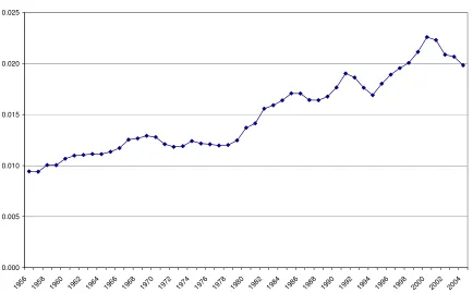
4. Calibration

Using the framework developed above, this section provides a quantitative assessment on the effects of

blocking patents. Figure 1 shows that in the US, private spending on R&D as a share of GDP has been

rising sharply since the beginning of the 80’s. Then, after a few years, the number of patents granted by

patent policy in the 80’s,8 the structural parameters are calibrated using long-run aggregate data of the

US’s economy from 1953 to 1980 to examine the extent of R&D underinvestment and the effects of

blocking patents before these policy changes. The goal of this numerical exercise is to quantify the effects

of eliminating blocking patents on R&D, consumption, welfare and capital investment.

4.1. Backloading Discount Factor

The first step is to calibrate the structural parameters and the steady-state value of the backloading

discount factor

ν

. The average annual TFP growth rate

g

_TFP is 1.33%,9 and the average labor-force

growth rate n is 1.94%.10 The annual depreciation rate

δ

on physical capital and the household’s discount

rate

ρ

are set to conventional values of 8% and 4% respectively. For the markup

µ

, Laitner and

Stolyarov (2004) estimate that the markup is about 1.1 (i.e. a 10% markup) in the US; on the other hand,

Basu (1996) and Basu and Fernald (1997) estimate that the aggregate profit share is about 3%. To be

conservative, I set

µ

to the lower value at 1.03.11 Some empirical studies have estimated the arrival rate

λ

of inventions, and I consider a wide range of values

λ

∈[0.04,0.20] that cover the usual estimates.12

(33) shows that holding other variables constant, an increase in

λ

must be offset by a decrease in

ν

to

hold the level of R&D constant. Therefore, at higher values of

λ

, the calibrated effects of blocking

patents would be even more severe.

For {

ν

,

α

,

σ

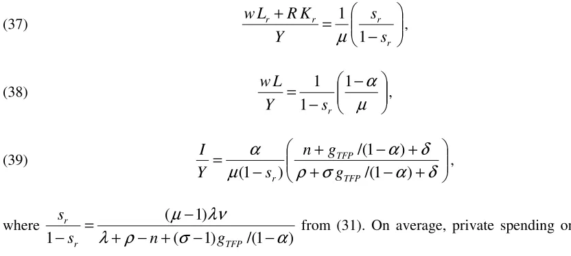
}, the model provides three steady-state conditions for the calibration (a) R&D share

of GDP in (37), (b) labor share in (38), and (c) capital-investment rate in (39).

8

See, for example, Jaffe (2000), Gallini (2002) and Jaffe and Lerner (2004) for a discussion.

9

Multifactor productivity for the private non-farm business sector is obtained from the Bureau of Labor Statistics.

10

The data on the annual average size of the labor force is obtained from the Bureau of Labor Statistics.

11

A higher markup would imply a more severe effect of blocking patents. Intuitively, a higher markup means increased profitability which must be offset by a stronger effect of blocking patents in order to hold the level of R&D in the data constant. In this case, eliminating blocking patents would lead to a more significant increase in R&D and consumption.

12

(37)

−

=

+

r r r r

s

s

Y

K

R

L

w

1

1

. .

µ

,

(38) −

− =

µ

α

1 1 1 . r s Y L w , (39)

+

−

+

+

−

+

−

=

δ

α

σ

ρ

δ

α

µ

α

)

1

/(

)

1

/(

)

1

(

. TFP

TFP r

g

g

n

s

Y

I

, where ) 1 /( ) 1 ( ) 1 (

1

λ

ρ

σ

α

λν

µ

− − + − + − =

− r TFP

r

g n

s s

from (31). On average, private spending on R&D as a

share of GDP is 0.0115.13 Labor share is set to a conventional value of 0.7, and the average ratio of

[image:22.612.70.486.73.260.2]

private investment to GDP is 0.203.14

Table 1 presents the calibrated values for the structural parameters along with the real interest rate

) 1 /(

.

α

σ

ρ

+ −

= gTFP

r for

λ

∈[0.04,0.40].

[image:22.612.119.495.375.463.2]

0.04 0.06 0.08 0.10 0.12 0.14 0.16 0.18 0.20 0.85 0.70 0.62 0.58 0.54 0.52 0.51 0.49 0.48 0.29 0.29 0.29 0.29 0.29 0.29 0.29 0.29 0.29 2.36 2.36 2.36 2.36 2.36 2.36 2.36 2.36 2.36 r 0.084 0.084 0.084 0.084 0.084 0.084 0.084 0.084 0.084

Table 1: Calibrated Structural Parameters

Table 1 shows that the calibrated values for {

α

,

σ

,r} are roughly invariant across different values of

λ

.

The calibrated value for the elasticity of intertemporal substitution (i.e. 1/

σ

) is about 0.42, which is

closed to the empirical estimates suggested by Guvenen (2006). The implied real interest rate is about

8.4%, which is slightly higher than the historical rate of return on the US’s stock market, and this higher

interest rate implies a lower socially optimal level of R&D spending in (34) and a higher steady-state

value of the backloading discount factor in (33). As a result, the model is less likely to overstate the extent

of R&D underinvestment and the degree of blocking patents. Furthermore, the fact that the calibrated

13

The data is obtained from the National Science Foundation and the Bureau of Economic Analysis. R&D is net of federal spending, and GDP is net of government spending. The data on R&D in 1954 and 1955 is not available.

14

values of

ν

∈[0.48,.0.85] are smaller than one suggests a severe degree of blocking patents in the US

economy. Therefore, reducing the extent of blocking patents may be an effective method to stimulate

R&D. After calibrating the externality parameters and computing the socially optimal level of R&D

spending, the effects of reducing the extent of blocking patents on consumption will be quantified.

4.2. Externality Parameters

The second step is to calibrate the values for the externality parameters

γ

(intratemporal duplication) and

φ

(intertemporal knowledge spillovers). To do this, I need to first determine the value of

g

_A by setting

TFP A g

g =

ξ

. for

ξ

∈[0,1]. The parameter

ξ

captures the fraction of long-run TFP growth driven by

R&D, and the remaining fraction is driven by the exogenous process Zt such that

g

Z

=

(

1

−

ξ

)

g

TFP. For

each value of

ξ

,

g

TFP,

n

, and

α

, the balanced-growth condition (30) determines a unique value for

) 1

/(

φ

γ

− , which is sufficient to determine the effects of R&D on consumption in the long run. However,

holding

γ

/(1−

φ

) constant, a larger

γ

implies a faster rate of convergence to the balanced-growth path.

Therefore, to determine the socially optimal level of R&D, it is important to consider different values of

γ

. To reduce the plausible parameter space of

γ

and

φ

, I make use of the empirical estimates for the

social rate of return to R&D. Following Jones and Williams’ (1998) derivation, Appendix C shows that

the net social rate of return r~ to R&D can be expressed as

(40) 1 1

1 1

~ _{+ + −}

+ +

=

γ

φ

r A A

Y

s g g

g

r .

After setting r~ to the lower bound of 0.30 as in Jones and Williams (1998, 2000), (30) and (40) pin down

a unique value of

γ

and

φ

for each value of

ξ

.

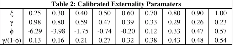
Table 2 presents the calibrated values of

γ

and

φ

for

ξ

∈[0.25,.1.0] that correspond to 0.3

~₌

r .

increases,

γ

/(1−

φ

) increases as shown in (30) and the intratemporal duplication effect can become more

severe while maintaining the social return of R&D in (40) at 0.3. When

ξ

equals 0.25, a social return of

0.3 implies that there must be negligible duplication externality. When all the TFP growth is driven by

R&D, the duplication effect can be as severe as

γ

=0.23.

[image:24.612.121.499.184.256.2]

0.25 0.30 0.40 0.50 0.60 0.70 0.80 0.90 1.00 0.98 0.80 0.59 0.47 0.39 0.33 0.29 0.26 0.23 -6.29 -3.98 -1.75 -0.74 -0.20 0.12 0.33 0.47 0.57 /(1- ) 0.13 0.16 0.21 0.27 0.32 0.38 0.43 0.48 0.54

Table 2: Calibrated Externality Paramaters

4.3. Socially Optimal Level of R&D Spending

This section calculates the socially optimal R&D share of GDP in (34). Figure 3 plots the socially optimal

R&D share for each set of parameter values in Table 2 that corresponds to r~ equal 0.30.

[insert Figure 3 here]

Figure 3 shows that there was underinvestment in R&D in the US over the entire range of parameters. In a

sense, this finding is not surprising given the large estimated social return to R&D. Optimal R&D share

increases in

ξ

in Figure 3 because a larger

ξ

implies a larger

γ

/(1−

φ

) in Table 2. Applying the log

approximation ln(1+x)≈x to (C4) and combining it with (34), it can be shown that

(41) −

− −

− + −

≈

− 1 1

1 ~

1 1

1 *

*

φ

γ

φ

γ

r Y Y r

r

s g r

g r s

s

.

Therefore, for a given social return ~r of R&D, s_r*/(1−s_r*) increases in

γ

/(1−

φ

) so long as r~>r.

4.4. Eliminating Blocking patents

Given the calibrated parameter values, this section quantifies the effects of eliminating blocking patents

on R&D and consumption. Table 3 shows that eliminating blocking patents (i.e. setting

ν

=1) would lead

the US would increase from 0.0115 in the data to a minimum of 0.0136 (i.e. an increase of 18%) in Table

3. For a large value of

λ

, R&D share of GDP may even double. Table 1 shows that the calibrated values

for

ν

decrease in

λ

; therefore, as

λ

increases, the increase in

ν

to eliminate blocking patents is larger

and hence leads to a more significant effect on R&D.

0.04 0.06 0.08 0.10 0.12 0.14 0.16 0.18 0.20 R&D 0.0136 0.0165 0.0185 0.0200 0.0211 0.0219 0.0226 0.0232 0.0237

Table 3: R&D Shares without Blocking Patents

Next, we quantify the effects of eliminating blocking patents on the level of consumption in the long run.

Along the balanced-growth path, per capita consumption increases at an exogenous rate gc. Therefore,

after dropping the exogenous growth path and some constant terms, long-run consumption can be derived

as a function of the steady-state value of the backloading discount factor

ν

through the

capital-investment rate i(

ν

) and the R&D share

s

r

(

ν

)

of factor inputs. It can be shown that in the case of a

change in

ν

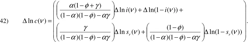
, the percent change in long-run consumption can be expressed as

(42) − ∆ − − − − + ∆ − − − + − ∆ + ∆ − − − + − = ∆ )) ( 1 ln( ) 1 )( 1 ( ) 1 ( ) ( ln ) 1 )( 1 ( )) ( 1 ln( ) ( ln ) 1 )( 1 ( ) 1 ( ) ( ln

ν

αγ

φ

α

φ

ν

αγ

φ

α

γ

ν

ν

αγ

φ

α

γ

φ

α

ν

r r s s i i c .

I consider the most conservative case that only one quarter of the TFP growth in the US is driven R&D

[image:25.612.76.506.399.472.2]

(i.e.

ξ

=0.25). A value of 0.25 for

ξ

implies a very small value of 0.13 for

γ

/(1−

φ

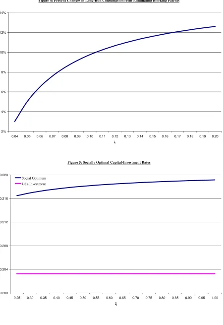
) in Table 2.15

Figure 4 shows that even in this conservative case, eliminating blocking patents would raise the

balanced-growth level of consumption by at least 3% (percent change) and up to over 12% if the change in

v

is

large enough. Also, the change in consumption mostly comes from

(

γ

/((

1

−

α

)(

1

−

φ

)

−

αγ

))

∆

ln

s

r

(

ν

)

in (42) that is the direct effect of R&D on consumption through technology; in other words, the other

general-equilibrium effects only have secondary impacts on long-run consumption.

[insert Figure 4 here]

15

In addition to examining the effects of blocking patents on long-run consumption, I also consider

the transition dynamic effects. I use the relaxation algorithm developed by Trimborn et al. (2008) to

compute the transition path of consumption.16 For the set of parameter values considered before (i.e.

25 . 0

=

ξ

in Table 2 and

λ

∈[0.04,.0.20] in Table 3), upon eliminating blocking patents, consumption

falls slightly on impact and then gradually rises to the new balanced-growth path.17 I use the consumption

path up to 100 years after the policy change to calculate the representative household’s utility (1) on this

new transition path and compare it to the household’s original utility on the old balanced-growth path.

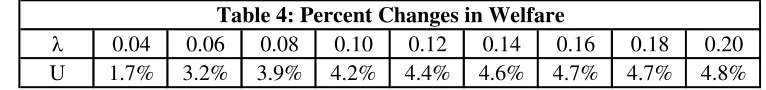
Table 4 reports the percent changes in welfare (i.e. the household’s lifetime utility).18

[image:26.612.111.494.278.323.2]

0.04 0.06 0.08 0.10 0.12 0.14 0.16 0.18 0.20 U 1.7% 3.2% 3.9% 4.2% 4.4% 4.6% 4.7% 4.7% 4.8%

Table 4: Percent Changes in Welfare

To have a sense on how important these changes are, an increase of 1.7% (4.8%) in the household’s

lifetime utility requires a permanent increase in consumption of 1.3% (3.7%).

4.5. Dynamic Distortion

Proposition 1 derives the condition under which the equilibrium rate of investment in physical capital is

below the socially optimal level. The following numerical exercise quantifies this wedge. Figure 5

presents the socially optimal rates of capital investment in (35) along with the US’s investment rate, and

the wedge is about 0.014 on average.

[insert Figure 5 here]

16

I would like to thank Timo Trimborn for his advice on the relaxation algorithm.

17

In fact, consumption does not necessarily fall on impact but instead gradually rises to the new balanced-growth path over a wide range of parameters that correspond to a higher social return to R&D (i.e. larger ξ, γ and φ). In other words, in a model with capital, it is possible for households to avoid short-run consumption losses by running down the capital stock, and this finding is different from models without capital accumulation. See, for example, Kwan and Lai (2003) for an interesting analysis on the transition dynamic effects of patent policy in a variety-expanding model without capital accumulation.

18

The equilibrium rate of investment in physical capital is increasing in the R&D share of capital.

Therefore, eliminating blocking patents also increases the capital-investment rate. Table 5 shows that

upon eliminating blocking patents, the steady-state capital-investment rate increases from 0.203 in the

data slightly toward the socially optimal level.

0.04 0.06 0.08 0.10 0.12 0.14 0.16 0.18 0.20 I/Y 0.204 0.204 0.205 0.205 0.205 0.205 0.206 0.206 0.206

Table 5: Capital-Investment Rates without Blocking Patents

4.6. Discussion

The numerical analysis is based on a number of calibrated parameters and variables. The key parameter is

ξ

and the key variable is

ν

. The calibrated values for

ξ

imply R&D underinvestment. A lower bound of

0.25 for

ξ

is based on the previous empirical estimates on the social return to R&D. If R&D has little

social values, then the actual value of

ξ

would be smaller and hence there may be no underinvestment in

R&D. However, even if R&D is not underinvested, reducing the extent of blocking patents would allow

the policymakers to lower the breadth (i.e. the markup) that reduces the distortionary effects of patent

policy while keeping the level of R&D constant.

The calibrated values for

ν

imply a significant effect of blocking patents. An upper bound of

0.85 for

ν

is based on a number of assumptions. The first assumption is that the data on R&D investment

is reasonably accurate. If there is a large amount of R&D spending not recorded, then the identification of

ν

using (33) would imply a downward bias on

ν

(i.e. an overestimate of blocking patents). Secondly,

applying (33) to aggregate data requires an assumption that monopolistic profits in the economy are

created by patent protection. To the extent that only a small fraction of profits is created by patent

protection, the identification of

ν

using (33) would also imply a downward bias on

ν

. However, using a

patent-protected and R&D-intensive industries, the markup and the profit share should be much larger.19 Thirdly,

when

λ

is below the lower bound of 0.04, (33) would indicate a less significant effect of blocking patents

(i.e. a larger

ν

). However, such a small value of

λ

implies that the average time between arrivals of

inventions would be longer than 25 years. On the other hand, for larger values of

λ

(e.g. Acemoglu and

Akcigit (2008) consider an average arrival rate

λ

of 0.33), the calibrated values for

ν

would be smaller

(i.e. an even more severe effect of blocking patents).

Finally, the numerical analysis is performed on a semi-endogenous growth model, in which

increasing R&D investment has no effect on long-run growth. In the case of a fully endogenous-growth

model, raising R&D through the elimination of blocking patents would increase the long-run growth rate

of consumption. For example, doubling R&D would increase the R&D-driven TFP growth rate by a

factor of 2γ in the first-generation quality-ladder growth models. So long as

ξ

and

γ

are not negligible,

this kind of increase in the long-run growth rate would have tremendous effects on welfare. Therefore, the

calibrated effects from a semi-endogenous growth model are likely to be conservative.

5. Conclusion

This paper has attempted to accomplish three objectives. Firstly, it develops a quantitative framework that

can be applied to evaluate the effects of blocking patents. Secondly, it applies the model to aggregate data

to perform hypothetical policy experiments. Thirdly, it identifies a dynamic distortionary effect of patent

policy on capital accumulation that has been neglected by previous studies. The numerical exercise

suggests the following findings. If a non-trivial fraction of TFP growth in the US is driven by R&D, there

is underinvestment in R&D in the economy. Then, provided that blocking patents have a significant and

negative effect on R&D, reducing this negative effect of overlapping intellectual property rights while

keeping its positive effect (i.e. patent breadth) constant can help mitigating the R&D-underinvestment

problem. The resulting increase in R&D could lead to a substantial increase in consumption.

19

The readers are advised to interpret the numerical results with some important caveats in mind.

The first caveat is that although the quality-ladder growth model has been generalized as an attempt to

capture more realistic features of the US economy, it is still an oversimplification of the real world.

Furthermore, the finding that eliminating blocking patents has substantial and positive effects on R&D

and consumption is based on the assumptions that the empirical estimates on the social return to R&D and

the data on R&D investment are reasonably accurate. The validity of these assumptions remains as an

empirical question.

Finally, I conclude this paper with some policy implications. The changes in patent policy in the

80’s are conventionally believed to include a broadening of patent breadth. The theoretical analysis

suggests that a broader patent breadth increases R&D at the costs of worsening the distortionary effects

on patent protection. In other words, there exists a welfare tradeoff using this policy instrument. On the

other hand, holding patent breadth constant, reducing the extent of blocking patents would stimulate R&D

without worsening the distortionary effects. This reasoning suggests that for the purpose of stimulating

R&D, reducing the extent of blocking patents would have been a less harmful policy instrument than

increasing patent breadth. Even if the current level of R&D is socially optimal, it would be beneficial for

the society to reduce the level of patent breadth and the extent of blocking patents simultaneously to keep

R&D constant. A lower level of patent breadth would reduce the distortionary effects of patent protection