Hybrid Neuro Fuzzy Controller for Automatic Generation Control of Multi Area Deregulated Power System

http://dx.doi.org/10.4236/cs.2016.74026

How to cite this paper: Solaiappan, B.S. and Kamaraj, N. (2016) Hybrid Neuro Fuzzy Controller for Automatic Generation Control of Multi Area Deregulated Power System. Circuits and Systems, 7, 292-306.

http://dx.doi.org/10.4236/cs.2016.74026

Hybrid Neuro Fuzzy Controller for

Automatic Generation Control of Multi

Area Deregulated Power System

Baghya Shree Solaiappan1*, Nagappan Kamaraj2

1_{Department of Electrical and Electronics Engineering, Anna University-University College of Engineering,}

Dindigul, India

2_{Department of Electrical and Electronics Engineering, Thiagarajar College of Engineering, Madurai, India}

Received 22 February 2016; accepted 24 April 2016; published 27 April 2016

Copyright © 2016 by authors and Scientific Research Publishing Inc.

This work is licensed under the Creative Commons Attribution International License (CC BY). http://creativecommons.org/licenses/by/4.0/

Abstract

This paper is intended in investigating the Automatic Generation Control (AGC) problem of a de-regulated power system using Adaptive Neuro Fuzzy controller. Here, three area control structure of Hydro-Thermal generation has been considered for different contracted scenarios under di-verse operating conditions with non-linearities such as Generation Rate Constraint (GRC) and Backlash. In each control area, the effects of the feasible contracts are treated as a set of new input signals in a modified traditional dynamical model. The key benefit of this strategy is its high in-sensitivity to large load changes and disturbances in the presence of plant parameter discrepancy and system nonlinearities. This newly developed scheme leads to a flexible controller with a sim-ple structure that is easy to realize and consequently it can be constructive for the real world power system. The results of the proposed controller are evaluated with the Hybrid Particle Swarm Optimisation (HCPSO), Real Coded Genetic Algorithm (RCGA) and Artificial Neural Network (ANN) controllers to illustrate its robustness.

Keywords

AGC, ANFIS, ANN, Deregulated Power System, HCPSO, RCGA

1. Introduction

the power flow. The escalation in size and convolution of electric power industry along with increase in power demand has necessitated the use of intelligent systems that combine knowledge, techniques and methodologies from various sources for the real-time control of power systems.

The electric power trade at present is largely in the hands of Vertically Integrated Utilities (VIU) which pos-sess generation, transmission and distribution systems facilitates to supply power to the customer at regulated tariff. The major revolutionize that has arisen be the emergence of Independent Power Producer (IPP) that can sell power to VIU. Given the present situation, it is generally agreed that the first step in deregulation will be to separate the generation of power from the transmission and distribution, thus putting all the generation on the same footing as the IPP. In an interconnected power system, a sudden load perturbation in any area causes the deviation of frequencies of all the areas and also in the tie-line powers. This has to be corrected to ensure the generation and distribution of electric power with good quality. This is accomplished by Automatic Generation Control (AGC). The main objectives of AGC [1][2] are to be maintained the desired MegaWatt output and the nominal frequency in an interconnected power system besides maintaining the net interchange of power between control areas at predetermined values. The AGC task is carried out through the error signal produced during generation and net interchange between the areas (i.e.,) Area Control Error (ACE) [3].

(

)

ACE tie i j i i j

P b f

=

∑

where bi be the frequency bias coefficient of the i th

area, ∆fi be the frequency error of the i th

area, ∆Ptie i j, , be the tie line power flow error between ith area and jth area.

With the restructuring of electric utilities, AGC requirements should be expanded to include the planning functions necessary to ensure the resources needed for AGC implementation are within the functional require-ments. So most of the methods that may be proposed must have a good ability to track the contracted or un-contracted demands and can be used in a practical environment. A lot of studies have been made about AGC in a restructured power industry over last decades. These studies try to modify the conventional LFC system [4] to take into account the effect of bilateral contracts on the dynamics [5] and improve the dynamical transient re-sponse of the system under competitive conditions [6]-[8]. This paper proposes a control scheme that guarantees a minimum transient deviation and ensures zero steady state error. The stabilization of frequency oscillations in an interconnected power system [9] becomes challenging when implements in the future competitive environ-ment. Consequently advanced economic, high efficiency and improved control schemes [10][11] are required to ensure the power system reliability. The conventional load-frequency controller may no longer be able to at-tenuate the large frequency oscillation due to the slow response of the governor [12][13]. A number of control strategies have been employed in the design of load frequency controllers in order to achieve better dynamic performance [13][14]. Among the various types of load frequency controllers, the most widely employed is the conventional proportional integral (PI) controller [13]-[15]. Conventional controller is simple for implementa-tion but takes more time and gives large frequency deviaimplementa-tion. A number of state feedback controllers based on linear optimal control theory have been proposed to achieve enhanced performance [16][17]. Fixed gain con-trollers are designed at nominal operating conditions and fail to provide best control performance over a wide range of operating conditions [18]. Subsequently, to keep system performance near its optimum, it is desirable to track the operating conditions and use updated parameters to compute the control. Adaptive controllers with self-adjusting gain settings have been proposed for LFC [17] [19]-[22].

There has also been considerable research work attempting to propose better AGC systems based on modern control theory [16], neural network [23]-[27] fuzzy system theory [19] and reinforcement learning [26]. Recent study confirms that ANFIS approach has also been applied to hydrothermal system [28]-[30]. All research dur-ing the earlier period in the area of AGC narrates interconnected two equal area thermal system and petite atten-tion has been paid to AGC of unequal multi area systems [31]. Most of ancient time works have been centred in the region of the design of governor secondary controllers, and design of governor primary control loop. Ap-parently no literature has discussed AGC performance subject to simultaneous small step load perturbations in all area or the application of ANFIS technique to a multi-area power system.

In this paper, an effort has been made to apply ANFIS controller for the automatic generation control for the three area hydro-thermal restructured power system in consideration with GRC and backlash.

2. System Analyzed

294

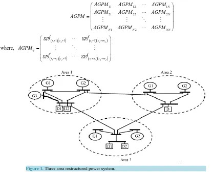
of GENCOs and DISCOs as shown in Figure 11. Area 1 comprises of three GENCOs with thermal power sys-tem of reheat and hydro turbine combinations and two DISCOs, Area 2 comprises of two GENCOs with hydro and thermal (reheat turbine) combination and one DISCO, Area 3 consists of two GENCOs with hydro and thermal (reheat turbine) combination and two DISCOs as shown in Figure 2.

In this restructured environment, any GENCO in one area may supply DISCOs in the same area as well as DISCOs in other areas. In other words, for restructured system having several GENCOs and DISCOs, any DISCO may contract with any GENCO in another control area independently by Bilateral Transaction. The transactions should be made through an independent system operator (ISO). The primary intention of ISO is to control many ancillary services, one of which is AGC. In open access scenario, any DISCO has the freedom to purchase MW power at competitive price from different GENCOs, which may or may not have contract with the same area as the DISCO. The contracts of GENCOs and DISCOs described by “DISCO participation matrix” (DPM). The DPM for the nth area power system is as follows:

11 12 1

21 22 2

1 2

n

n

n n nn

cpf cpf cpf

cpf cpf cpf

DPM

cpf cpf cpf

      =              (2)

In DPM, the number of rows is equal to the number of GENCOs and the number of columns is equal to the number of DISCOs in the system. Any entry of this matrix is a fraction of total load power contracted by a DISCO towards a GENCO [24]. The sum of total entries in a column corresponds to one DISCO be equal to one

(i.e.,) 1 1 n ij j cpf = =

∑

11 12 1

21 22 2

1 2

N

N

N N NN

AGPM AGPM AGPM

AGPM AGPM AGPM

AGPM

AGPM AGPM AGPM

      =_{ }            (3) where, ( )( ) ( )( ) ( )( ) ( )( )

1 1 1

1

i j i j j

i i j i i j j

s z s z m

ij

s n z s n z m

gpf gpf AGPM gpf gpf + + + + + + + +       =           

Figure 1. Three area restructured power system.

Figure 2. Three area multi source power system structure.

For i j, =1, 2,,N, and

1

1

i

i i

k

s n

−

=

=

∑

1

1

j

j j

k

z m

−

=

296

GENCOs and DISCOs in area i. The gpfij refer to generation participation factor and shows the participation as-pect of GENCOi in total load following the requirement of DISCOj based on the possible contract.

The Augmented Generation Participation Matrix (AGPM), which depicts (3) the effective participation of DISCO with various GENCOs in all the areas with nonlinearities. The Sum of all entries in each column of AGPM is unity. To demonstrate the effectiveness of the modeling strategy and proposed control design, a three control area power system is considered with nonlinearities. While there are many GENCOs in each area, the ACE signal has to be distributed among them due to their ACE participation factor in the AGC task.

The scheduled contracted power exchange is given [13]:

, , scheduled tie i j P

∆ = (Demand of DISCOs in area 2 from GENCOs In area 1)-(Demand of DISCOs in area 1 from GENCOs in area 2)

Disturbance in ith area, di= ∆Ploc i, + ∆Pdi

where, , 1 i

m

loc i Lj i j

P P −

= ∆ =

∑

j

P P ₋

=

∆ =

∑

Area Interface for ith area,

1, N

i ij j

j j i T f η

= ≠

=

∑

Scheduled power tie line power flow deviation,

, , , ,

1, mj

i tie ik sch tie ik sch k k i

P P

ξ

= ≠

= ∆

∑

( )( ) ( )( ) , ,

1 1 1 1

i k k i

i k k i

n m n m

tie ik sch s j z t Lt k s t z j Lj k

j t t j

P apf _{+ +} P ₋ apf _{+ +} P ₋

= = = =

∆ =

∑∑

∑∑

, , ,

tie i error tie i actual i

P P ₋ ξ

∆ = ∆ − (8)

T

1 i

i i ki n i

ρ _{= }ρ _ρ _ρ _ (9)

( )( ) 1 1 j i j T m N

ki s k z t Lt j

j t

gpf P

ρ + + −

= =   = _ ∆ _  

∑ ∑

j

P P apf P ₋

=

∆ = +

∑

where k=1, 2,,ni

where k=1, 2,,ni and ∆Pm k i, , is the desired total power generation of a GENCO k in area i, moreover should track the demand of the DISCOs in contract with it in the steady state.

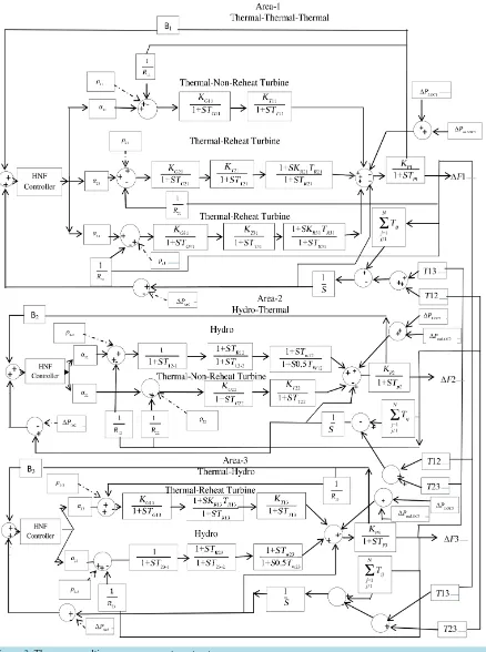
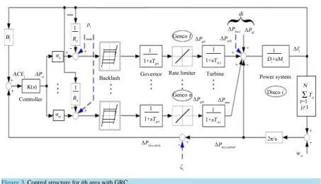
In a power system having steam plants, power generation can change only at a specified maximum rate. The structure for ith area in the presence of GRC is shown in Figure 3. A typical value of the generation rate con-straint (GRC) for thermal unit is 3%/min, i.e., GRC for the thermal system is ∆PGt t

( )

Two limiters, bounded by ±0.0005 are employed within the AGC of the thermal system to prevent the excessive control action. Likewise, for hydro plant GRC of 270%/min. for raising generation and 360%/min. for lowering generation has been deemed. Thus, for Raising, ∆PGh t

( )

( )

PGh t

∆ ≤ . The generation rate constraints for all the areas have been engaged keen on adding limiters to the turbines.

Figure 3. Control structure for ith area with GRC.

connecting the piston to the camshaft [23]. Backlash is the nonlinearity which causes governor dead band and tends to produce continuous sinusoidal oscillations with a natural period of about 2 secs.

3. ANFIS Approach

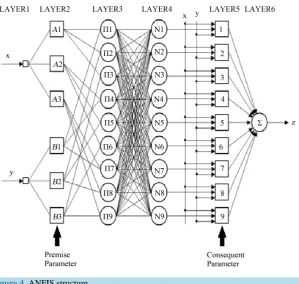
The Hybrid combination of neural and fuzzy is considered to be an adaptive network, which has no synaptic weights, however they have adaptive and non-adaptive nodes. The adaptive network can be simply transformed to neural network architecture with classical feed forward topology. This proposed network is functioning very similar to adaptive network simulator of Takagi-Sugeno’s fuzzy controllers. This adaptive network is operation-ally comparable to a fuzzy inference system (FIS). ANFIS adjusts the entire parameters using back propagation gradient descent and least squares type of method for non-linear and linear parameters, respectively by the pro-vided set of input/ output data [23][28]. The fuzzy reasoning is expressed as Rule 1: If x is A1 and y is B1, then

1 1 1 1

Z = p x+q y+r .

Figure 4 shows a 2-input, type-3 ANFIS with 9 rules. Three membership functions are associated with each

input, so the input space is partitioned into 9 fuzzy subspaces, each of which is governed by fuzzy if-then rules. The premise part of a rule defines a fuzzy subspace, while the consequent part specifies the output within this fuzzy subspace. The node functions in the same layer are of the same function family as described below. Layer 1 is the input layer. Neurons in this layer simply pass external crisp signals to Layer 2. Layer 2 is the fuzzifica-tion layer. Neurons in this layer perform fuzzificafuzzifica-tion based on Gaussian membership funcfuzzifica-tion. If x be the input to node i, and Ai is the linguistic associated with this node function. In other words,

1

i

O is the membership function of Ai and it indicates the degree to which the given x satisfies the measure Ai. Layer 3 is the rule layer. Each neuron in this layer corresponds to a single Sugeno-type fuzzy rule. A rule neuron receives inputs from the respective fuzzification neurons and calculates the firing strength of the rule it represents. In an ANFIS, the conjunction of the rule antecedents is evaluated by the operator product. Layer 4 is the normalisation layer. Each neuron in this layer receives inputs from all neurons in the rule layer, and calculates the normalised firing strength of a given rule. The normalised firing strength is the ratio of the firing strength of a given rule to the sum of firing strengths of all rules. It represents the contribution of a given rule to the final result.

298

Figure 4. ANFIS structure.

Layer 6 is represented by a single summation neuron. This neuron calculates the sum of outputs of all defuzzifi-cation neurons and produces the overall ANFIS output, z.

The Multi Layer Perceptron (MLP) structure model of ANN is exercised for AGC of three unequal area Hy-dro-Thermal system. Examinations has confirmed that ANNs have a broad number of application in the power engineering due to many virtues [29][30] such as capability of synthesize multifaceted and discernible planning, briskness due to parallel mechanism, robustness and fault forbearance.

In this article, ANFIS controller in MATLAB/Simulink, which is an advance adaptive control configuration of ANN, has been proposed. The proposed ANN controller uses back propagation through-time algorithm. The back-propagation technique is an iterative method employing the gradient decent algorithm for minimizing the minimum square error between the actual output and the objective for each pattern in the training. Then update the network weights in a recursive algorithm starting from the output layer and working backward to the first hidden layer. The learning process of ANFIS system acquires the semantically properties of the underlying fuzzy system into account. The ANFIS system consists of the components of a conventional fuzzy system ex-cept that computation at every phase is carried out by a layer of hidden neurons and the neural network’s learn-ing capacity is offered to boost the system knowledge.

ANFIS Controller Design

This ANFIS controller make use of Sugeno-type fuzzy inference system (FIS) controller, with the parameters surrounded by the FIS determined by the neural-network back propagation method. The ANFIS controller is de-signed by taking ACE and its derivative (d(ACE)/dt) as the inputs. The output stabilizing signal is worked out by using the fuzzy membership functions depending on these variables. ANFIS-Editor is used for realizing the system and for putting into practice. The fuzzy controller employs 49 rules and 7 membership functions in each variable to resolve output.

The procedure for designing ANFIS controller in MATLAB Simulink is as follows:

1) Sketch the Simulink model with fuzzy controller and simulate it with the specified rule base. 2) Collect the training data while simulating the model.

4) Use anfisedit to generate the ANFIS.fis file.

5) Stack the training data composed in Step 2 and create the FIS with Gaussian membership function. 6) Train the collected data with generate FIS up to a particular no. of Epochs.

7) Save the FIS. This FIS file is the Neuro-Fuzzy enhanced ANFIS file.

4. Simulation Results and Discussion

The AGC problem of three area deregulated power system is considered here with the non-linearities. Hybrid combinations of Neuro and fuzzy is used as a controller to evaluate frequency and tie-line responses of multi source power system. The simulations are carried out for the possible electricity contracts and also for large de-mand variations using HCPSO, RCGA, ANN controllers and the results were compared. Table 1 depicts tie line power deviations for all the scenarios using the various controllers. The values show that the tie line power ex-change between the areas, ANFIS controller reaches the exact exex-change of power between the areas with mini-mum deviations compared to other controllers. Table 2 shows the comparison of GENCO power deviation for the three scenarios with theoretical and the simulated values by Equation (10). In this ANFIS accomplish its controller task perfectly in getting the same value as it gains in theoretical calculation. The plant parameters for three area deregulated power system used for modeling the control structure is presented in Table 3. The results illustrate that proposed controller proves good dynamic performance over the others in terms of settling time, overshoot and undershoot (Table 4 and Table 5).

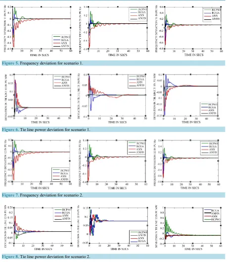
4.1. Scenario 1 Poolco Based Transactions

In this scenario, GENCOs take part only in the load pursuing the control of their areas. The transaction among DISCOs and available GENCOs is being simulated based on the following AGPM by Equation (3). The varia-tions in tie line power flows and frequency is shown in Figure 5 and Figure 6 and the values are depicted in

Table 4 and Table 5. The figures show that ANFIS controller secure the steady state deviation (Marked as

Black colour) with minimum settling time and reduced overshoot and undershoot.

0.3 0.25 0 0 0

0.4 0.35 0 0 0

0.3 0.4 0 0 0

0 0 0.5 0 0

0 0 0.5 0 0

0 0 0 0.45 0.6

0 0 0 0.55 0.4

AGPM

 

 

 

 

 

=  

 

 

 

 

 

Table 1. Tie line power deviation (pu MW).

Controller Scenario AREA

1 - 2 2 - 3 3 - 1

RCGA

1 −0.00047 −0.00044 0.0009

2 0.014991 0.07499 −0.09

3 0.014995 0.075 −0.09

HCPSO

1 7.30E−06 −3.60E−09 −7.00E−06

2 0.01494 0.074946 −0.0899

3 0.01492 0.074923 −0.0837

ANN

1 6.80E−06 −8.80E−06 −1.10E−06

2 0.01477 0.07499 −0.08559

3 0.01811 0.07492 −0.08985

ANFIS

1 −0.0014 0.00011 −0.0014

2 0.01488 0.075 −0.0853

300

Table 2. GENCO power deviations in pu Mw.

Test System Scenario Theoretical value

Value obtained through Simulation

ANFIS RCGA HCPSO ANN

Area 1

GENCO 1-Thermal with non-Reheat Turbine

1 0.055 0.055 0.055 0.055 0.055

2 0.065 0.065 0.065 0.065 0.065

3 0.085 0.085 0.085 0.085 0.085

GENCO 2 Thermal with Reheat Turbine

1 0.075 0.075 0.075 0.075 0.075

2 0.07 0.08 0.08 0.08 0.08

3 0.085 0.85 0.085 0.085 0.085

GENCO 3 Thermal with Reheat Turbine

1 0.07 0.07 0.07 0.07 0.07

2 0.08 0.08 0.08 0.08 0.08

3 0.095 0.095 0.095 0.095 0.095

Area 2

GENCO 1 Hydro

1 0.055 0.05 0.05 0.05 0.05

2 0.12 0.12 0.12 0.12 0.12

3 0.144 0.144 0.1439 0.144 0.144

GENCO 2 Thermal with non-Reheat Turbine

1 0.05 0.05 0.05 0.05 0.05

2 0.055 0.055 0.055 0.055 0.055

3 0.071 0.071 0.071 0.071 0.071

Area 3

GENCO 1 Thermal with reheat turbine

1 0.105 0.105 0.105 0.105 0.105

2 0.065 0.065 0.065 0.065 0.065

3 0.144 0.144 0.1439 0.144 0.144

GENCO 2 Hydro

1 0.095 0.095 0.095 0.095 0.095

2 0.045 0.045 0.045 0.045 0.045

3 0.06 0.06 0.0618 0.06 0.062

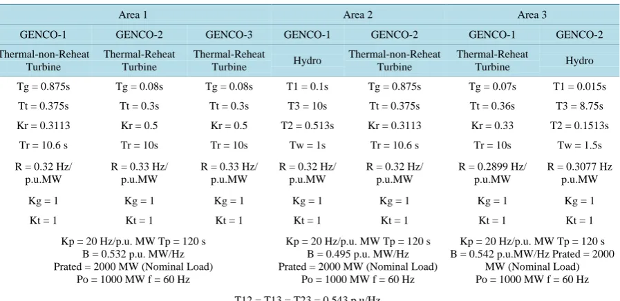
Table 3. Power system plant and control parameters.

Area 1 Area 2 Area 3

GENCO-1 GENCO-2 GENCO-3 GENCO-1 GENCO-2 GENCO-1 GENCO-2

Thermal-non-Reheat Turbine

Thermal-Reheat Turbine

Thermal-Reheat

Turbine Hydro

Thermal-non-Reheat Turbine

Thermal-Reheat

Turbine Hydro

Tg = 0.875s Tg = 0.08s Tg = 0.08s T1 = 0.1s Tg = 0.875s Tg = 0.07s T1 = 0.015s

Tt = 0.375s Tt = 0.3s Tt = 0.3s T3 = 10s Tt = 0.375s Tt = 0.36s T3 = 8.75s

Kr = 0.3113 Kr = 0.5 Kr = 0.5 T2 = 0.513s Kr = 0.3113 Kr = 0.33 T2 = 0.1513s

Tr = 10.6 s Tr = 10s Tr = 10s Tw = 1s Tr = 10.6 s Tr = 10s Tw = 1.5s

R = 0.32 Hz/ p.u.MW

R = 0.33 Hz/ p.u.MW

R = 0.33 Hz/ p.u.MW

R = 0.32 Hz/ p.u.MW

R = 0.32 Hz/ p.u.MW

R = 0.2899 Hz/ p.u.MW

R = 0.3077 Hz p.u.MW

Kg = 1 Kg = 1 Kg = 1 Kg = 1 Kg = 1 Kg = 1 Kg = 1

Kt = 1 Kt = 1 Kt = 1 Kt = 1 Kt = 1 Kt = 1 Kt = 1

Kp = 20 Hz/p.u. MW Tp = 120 s B = 0.532 p.u. MW/Hz Prated = 2000 MW (Nominal Load)

Po = 1000 MW f = 60 Hz

Kp = 20 Hz/p.u. MW Tp = 120 s B = 0.495 p.u. MW/Hz Prated = 2000 MW (Nominal Load)

Po = 1000 MW f = 60 Hz

Kp = 20 Hz/p.u. MW Tp = 120 s B = 0.542 p.u.MW/Hz Prated = 2000

MW (Nominal Load) Po = 1000 MW f = 60 Hz

Table 4. Tie line power deviation with respect to response characteristics.

Tie line power Deviations (pu MW)

Controller Area

Overshoots (MW) Undershoot (MW) Settling time (secs)

Scenario Scenario Scenario

1 2 3 1 2 3 1 2 3

HCPSO

1 - 2 0.1204 0.1185 0.141 −0.008 −0.058 −0.1 9 16 15

2 - 3 0.0946 0.1393 0.193 −0.004 −0.006 −0.026 9 14 14

3 - 1 0.0009 0.037 0.0523 −0.212 −0.253 −0.305 10 14 16

RCGA

1 - 2 0.1653 0.1261 0.1394 −0.034 −0.008 −0.007 12 18 19

2 - 3 0.0937 0.111 0.1324 −0.075 0 0 13 18 21

3 - 1 0.0987 0 0 −0.248 −0.237 −0.271 14 18 26

ANN

1 - 2 0.1685 0.1724 0.2082 −0.01 −0.01 −0.016 11 28 31

2 - 3 0.0907 0.1122 0.1324 −0.013 −0.006 0 26 26 33

3 - 1 0.0079 0 0 −0.214 −0.222 −0.248 27 25 28

ANFIS

1 - 2 0.052 0.0266 0.048 −0.044 −0.019 −0.136 4 9 14

2 - 3 0.0037 0.1393 0.1092 −0.012 −0.006 −0.007 5 12 13

3 - 1 0.052 0.6619 0.0523 −0.044 −0.085 −0.156 6 13 12

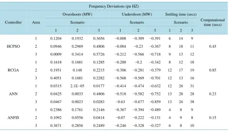
Table 5. Frequency deviation with respect to response characteristics.

Frequency Deviations (pu HZ)

Controller Area

Overshoots (MW) Undershoot (MW) Settling time (secs)

Computational time (secs)

Scenario Scenario Scenario

1 2 3 1 2 3 1 2 3

HCPSO

1 0.1204 0.1932 0.3656 −0.008 −0.309 −0.391 6 14 9

0.45 2 0.0946 0.2969 0.4806 −0.004 −0.23 −0.367 8 18 11

3 0.0009 0.3414 0.5726 −0.212 −0.566 −0.718 9 13 12

RCGA

1 0.1618 0.1681 0.1285 −0.288 −0.2 −0.342 8 12 18

0.85 2 0.1951 0.148 0.2215 −0.306 −0.281 −0.379 12 17 19

3 0.4051 0.1681 0.2282 −0.568 −0.569 −0.701 12 13 16

ANN

1 0.0315 2.1E−05 0.0177 −0.414 −0.474 −0.632 12 26 31

0.23 2 0.0425 0.0033 0.4806 −0.518 −0.582 −0.752 13 28 28

3 0.0467 0.0023 0.0283 −0.63 −0.677 −0.859 13 26 38

ANFIS

1 0.2386 0.1761 0.2146 −0.367 −0.394 −0.489 4 8 9

0.15 2 0.1092 0.0556 0.0414 −0.07 −0.222 −0.131 4 9 8

3 0.3671 0.2856 0.2489 −0.246 −0.328 −0.327 6 8 10

4.2. Scenario 2 Synthesis of Poolco and Bilateral Based Transactions

In this case, DISCOs have the liberty to deal with any of the GENCOs within or with other areas. The AGC as-signment accomplished through the following AGPM. The inconsistency based on this transaction is shown in

Figure 7 and Figure 8 prevailing to frequency and tie line power deviations (Table 4 and Table 5). The

302

Figure 5. Frequency deviation for scenario 1.

Figure 6. Tie line power deviation for scenario 1.

Figure 7. Frequency deviation for scenario 2.

Figure 8. Tie line power deviation for scenario 2.

0.2 0.15 0.1 0 0.2

0.25 0.2 0 0.1 0.15

0.1 0 0.3 0.25 0.15

0.3 0.15 0.3 0.25 0.2

0 0.2 0 0.15 0.2

0.15 0.2 0.15 0.15 0

0 0.1 0.15 0.1 0.1

AGPM

 

 

 

 

 

=  

 

 

 

 

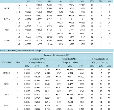
4.3. Scenario 3 Contract Violation

In this scenario, the DISCOs may defy the contracts by demanding more power than that stated in the contract. This excessive power is revealed as a located load of that area (un- contracted demand). This case has been car-ried out for various demand condition such as 10%, 20% and 30% which is depicted in Table 6 and Table 7. In all the load disturbances cases, ANFIS gains a good performance measures. The intention of this scenario is to test the effectiveness of the proposed controller against the uncertainties and sudden large load disturbances in the presence of GRC and backlash. Figure 9 and Figure 10 show the 10% rise in demand (presented in Table 4

and Table 5) of discos in all the three areas. The characteristics thus derived demonstrate that ANFIS is being a

best one to provide the steady state deviations with minimum overhooot, undershoot and also it settles quickly compared to other controllers.

Table 6. Tie line power deviation for load change.

Tie line power Deviations (pu MW)

Controller Area

Overshoots (MW) Undershoot (MW) Settling time (secs)

Change in Load (+) Change in Load (+) Change in Load (+)

10% 20% 30% 10% 20% 30% 10% 20% 30%

HCPSO

1 - 2 0.141 0.1635 0.186 −0.1 −0.142 −0.184 15 16 16

2 - 3 0.193 0.2467 0.3004 −0.026 −0.046 −0.066 14 17 15

3 - 1 0.0523 0.0676 0.0829 −0.305 −0.357 −0.409 16 17 18

RCGA

1 - 2 0.1394 0.1527 0.166 −0.007 −0.008 −0.009 19 19 19

2 - 3 0.1324 0.1538 0.1752 0 0 0 21 21 23

3 - 1 0 0 0 −0.271 −0.305 −0.339 26 26 26

ANN

1 - 2 0.2082 0.244 0.2798 −0.016 −0.022 −0.028 31 32 31

2 - 3 0.1324 0.1526 0.1728 0 0.006 0.012 33 33 33

3 - 1 0 0 0 −0.248 −0.274 −0.3 28 31 30

ANFIS

1 - 2 0.048 0.0694 0.0908 −0.136 −0.253 −0.37 14 14 15

2 - 3 0.1092 0.0791 0.049 −0.007 −0.008 −0.009 13 13 13

3 - 1 0.0523 −0.557 −1.166 −0.156 −0.227 −0.298 12 12 12

Table 7. Frequency deviation for load change.

Frequency Deviations (pu HZ)

Controller Area

Overshoots (MW) Undershoot (MW) Settling time (secs)

Change in Load (+) Change in Load (+) Change in Load (+)

10% 20% 30% 10% 20% 30% 10% 20% 30%

HCPSO

1 0.3656 0.538 0.7104 −0.391 −0.473 −0.555 15 16 16

2 0.4806 0.6643 0.848 −0.367 −0.504 −0.641 14 17 15

3 0.5726 0.8038 1.035 −0.718 −0.87 −1.022 16 17 18

RCGA

1 0.1285 0.0889 0.0493 −0.342 −0.484 −0.626 19 19 19

2 0.2215 0.295 0.3685 −0.379 −0.477 −0.575 21 21 23

3 0.2282 0.2883 0.3484 −0.701 −0.833 −0.965 26 26 26

ANN

1 0.0177 0.0354 0.0531 −0.632 −0.79 −0.948 31 32 31

2 0.4806 0.9579 1.4352 −0.752 −0.922 −1.092 33 33 33

3 0.0283 0.0543 0.0803 −0.859 −1.041 −1.223 28 31 30

ANFIS

1 0.2146 0.2531 0.2916 −0.489 −0.584 −0.679 14 14 15

2 0.0414 0.0272 0.013 −0.131 −0.04 0.051 13 13 13

304

Figure 9. Frequency deviation for scenario 3.

Figure 10. Tie line power deviation for scenario 3.

The Deviation in tie line power flows for these possible contracts are presented in Table 4. The results thus obtained through simulation depicts that the proposed ANFIS controller holds good performance as compared to RCGA, HCPSO and ANN controllers for all possible contracts and for wide range of load disturbances.

5. Conclusion

Adaptive Neuro Fuzzy approach is employed to AGC problem in deregulated power system. The proposed con-troller proves its capability in organizing the different areas of deregulated power system in the presence of non- linearites. This controller achieves reliability over tracking frequency and tie line power deviations for a wide range of load disturbances and system uncertainties. The simulation result carves out its robust performance with reduced overshoot, undershoot and settling time while compared to RCGA, HCPSO and ANN controllers. The Artificial Intelligence has bench marked its effectiveness in Automatic Generation Control and it is best suitable for real time power system to get online coordination for the deregulated environment.

References

[1] Bevrani, H., Mitani, Y. and Tsuji, K. (2004) Robust Decentralized AGC in a Restructured Power System. Energy

Conversion and Management, 45, 2297-2312. http://dx.doi.org/10.1016/j.enconman.2003.11.018

[2] Ibrabeem, P.K. and Kothari, D.P. (2005) Recent Philosophies of Automatic Generation Control Strategies in Power Systems. IEEE Transactions on Power Systems, 20, 346-357. http://dx.doi.org/10.1109/TPWRS.2004.840438

[3] Elgerd, O.I. (1971) Electric Energy Systems Theory. McGraw-Hill, New York, 315-389.

[4] Yousef, M.Z., Jain, P.K. and Mohamed, E.A. (2003) A Robust Power System Stabilizer Configuration Using Artificial Neural Network Based on Linear Optimal Control. Canadian Conference Electrical and Computer Engineering, 1, 569-573.

[5] Bevrani, H., Mitani, Y., Tsuji, K. and Bevrani, H. (2005) Bilateral Based Robust Load Frequency Control. Energy

Conversion and Management, 46, 1129-1146. http://dx.doi.org/10.1016/j.enconman.2004.06.024

[6] Menniti, D., Pinnarelli, A. and Scordino, N. (2004) Using a FACTS Device Controlled by a Decentralized Control Law to Damp the Transient Frequency Deviation in a Deregulated Electric Power System. Electric Power Systems Research,

72, 289-298. http://dx.doi.org/10.1016/j.epsr.2004.04.013

[7] Tan, W. and Xu, Z. (2009) Robust Analysis and Design of Load Frequency Controller for Power Systems. Electric

Power Systems Research, 79, 846-853. http://dx.doi.org/10.1016/j.epsr.2008.11.005

[9] Kirchmayer, L.K. (1959) Economic Control of Interconnected Systems. Wiley, New York.

[10] Bhatt, P., Roy, R. and Ghoshal, S. (2010) Optimized Multi Area AGC Simulation in Restructured Power Systems.

In-ternational Journal of Electrical Power & Energy Systems, 32, 311-322. http://dx.doi.org/10.1016/j.ijepes.2009.09.002

[11] Rakhshani, E. and Sadeh, J. (2010) Practical Viewpoints on Load Frequency Control Problem in a Deregulated Power System. Energy Conversion and Management, 51, 1148-1156. http://dx.doi.org/10.1016/j.enconman.2009.12.024

[12] Abraham, R.J., Das, D. and Patra, A. (2011) Load Following in a Bilateral Market with Local Controllers.

Internation-al JournInternation-al of ElectricInternation-al Power & Energy Systems, 33, 1648-1657. http://dx.doi.org/10.1016/j.ijepes.2011.06.033

[13] Tan, W. (2011) Decentralized Load Frequency Controller Analysis and Tuning for Multi-Area Power Systems. Energy

Conversion and Management, 52, 2015-2023. http://dx.doi.org/10.1016/j.enconman.2010.12.011

[14] Ansarian, M., Shakouri, H., Nazarzadeh, G.J. and Sadeghzadeh, S.M. (2006) A Novel Neuro Optimal Approach for

LFC Decentralized Design in Multi-Area Power System. 2006 IEEE International Power and Energy Conference,

Pu-tra Jaya, 28-29 November 2006, 167-172. http://dx.doi.org/10.1109/pecon.2006.346640

[15] Ram, P. and Jha, A.N. (2010) Automatic Generation Control of Interconnected Hydrothermal System in Deregulated

Environment Considering Generation Rate Constraints. 2010 International Conference on Industrial Electronics,

Con-trol & Robotics (IECR), Orissa, 27-29 December 2010, 148-159. http://dx.doi.org/10.1109/IECR.2010.5720143

[16] Khuntia, S.R. and Panda, S. (2010) Comparative Study of Different Controllers for Automatic Generation Control of an Interconnected Hydro-Thermal System with Generation Rate Constraints. 2010 International Conference on

Indus-trial Electronics, Control & Robotics (IECR), Orissa, 27-29 December 2010, 243-246.

http://dx.doi.org/10.1109/iecr.2010.5720151

[17] Tan, W. (2010) Unified Tuning of PID Load Frequency Controller for Power Systems via IMC. IEEE Transactions on

Power Systems, 25, 341-350. http://dx.doi.org/10.1109/TPWRS.2009.2036463

[18] Ghoshal, S.P. and Goswami, S.K. (2003) Application of GA Based Optimal Integral Gains in Fuzzy Based Active Power-Frequency Control of Non-Reheat and Reheat Thermal Generating Systems. Electric Power Systems Research,

67, 79-88. http://dx.doi.org/10.1016/S0378-7796(03)00087-7

[19] Tan, W. (2009) Tuning of PID Load Frequency Controller for Power Systems. Energy Conversion and Management,

50, 1465-1472. http://dx.doi.org/10.1016/j.enconman.2009.02.024

[20] Gomez, A.F., Delgado, M. and Vila, M.A. (1999) About the Use of Fuzzy Clustering Techniques for Fuzzy Model Identification. Fuzzy Sets and Systems, 106, 179-188. http://dx.doi.org/10.1016/S0165-0114(97)00276-5

[21] Shayeghi, H., Shayanfar, H.A. and Jalili, A. (2006) Multi-Stage Fuzzy PID Power System Automatic Generation Con-troller in Deregulated Environments. Energy Conversion and Management, 47, 2829-2845.

http://dx.doi.org/10.1016/j.enconman.2006.03.031

[22] Shayeghi, H. and Shayanfar, H.A. (2006) Decentralized Robust AGC Based on Structured Singular Values. Journal of

Electrical Engineering, 57, 305-317.

[23] Demiroren, A. and Zeynelgil, H.L. (2007) GA Application to Optimization of AGC in Three Area Power System after

Deregulation. International Journal of Electrical Power & Energy Systems, 29, 230-240.

http://dx.doi.org/10.1016/j.ijepes.2006.07.005

[24] Wu, Q.H., Hogg, B.W. and Irwin, G.W. (1992) A Neural Network Regulator for Turbo Generator. IEEE Transactions

on Neural Networks, 3, 95-100. http://dx.doi.org/10.1109/72.105421

[25] Beaufays, F., Magid, Y.A. and Widrow, B. (1994) Application of Neural Network to Load Frequency Control in Power System. IEEE Transactions on Neural Networks, 7, 183-194. http://dx.doi.org/10.1016/0893-6080(94)90067-1

[26] Chaturvedi, D.K., Satsangi, P.S. and Kalra, P.K. (1999) Load Frequency Control: A Generalized Neural Network Ap-proach. International Journal of Electrical Power & Energy Systems, 21, 405-415.

http://dx.doi.org/10.1016/S0142-0615(99)00010-1

[27] Zeynelgil, H.L., Demiroren, A. and Sengor, N.S. (2002) The Application of ANN Technique to Automatic Generation

Control for Multi-Area Power System. International Journal of Electrical Power & Energy Systems, 24, 345-354.

http://dx.doi.org/10.1016/S0142-0615(01)00049-7

[28] Hosseini, S.H. and Etemadi, A.H. (2008) Adaptive Neuro-Fuzzy Inference System Based Automatic Generation

Con-trol. Electric Power Systems Research, 78, 1230-1239. http://dx.doi.org/10.1016/j.epsr.2007.10.007

[29] Rao, C.S. (2010) Adaptive Neuro-Fuzzy Based Inference System for Load Frequency Control of Hydrothermal System

under Deregulated Environment. International Journal of Engineering Science and Technology, 2, 6954-6962. [30] Rojas, I., Bernier, J.L., Rodriguez-Alvarez, R. and Prieto, Z. (2010) What Are the Main Functional Blocks Involved in

the Design of Adaptive Neuro-Fuzzy Inference Systems. Proceedings of the IEEE-INNS-ENNS International Joint

Conference on Neural Networks, 6, 551-556. http://dx.doi.org/10.1109/ijcnn.2000.859453

[31] Ramey, D.G. and Skooglund, J.W. (1970) Detailed Hydro Governor Representation for System Stability Studies. IEEE

306

Nomenclature

i subscript referred to area F Area frequency

Ptie tie line power flow PT turbine power

PV governor valve position PC governor set point ACE area control error

cpf contract participation factor gpf generation participation factor KP subsystem equivalent gain constant TP subsystem equivalent time constant TT turbine time constant

TG governor time constant R droop characteristic B frequency bias FD Frequency Deviation

Tij tieline synchronizing coefficient between areas i&j Pd area load disturbance

PLji contracted demand of DISCO j in area i PULji un-contracted demand of DISCO j in area i PM,ji power generation of GENCO j in area i PLoc total local demand

η Area interface

ξ Scheduled power tie line power flow deviation GRC Generation Rate Constraint