Munich Personal RePEc Archive
Predicting Elections from Biographical
Information about Candidates
Armstrong, J. Scott and Graefe, Andreas
23 June 2009
Online at
https://mpra.ub.uni-muenchen.de/17709/
Predicting Elections from Biographical Information about Candidates
We seek peer review for this paper.
J. Scott Armstrong
The Wharton School
University of Pennsylvania, Philadelphia, PA
Andreas Graefe
Institute for Technology Assessment and Systems Analysis Karlsruhe Institute of Technology, Germany
October 7, 2009
Abstract. Using the index method, we developed the PollyBio model to predict election outcomes. The model, based on 49 cues about candidates’ biographies, was used to predict the
outcome of the 28 U.S. presidential elections from 1900 to 2008. In using a simple heuristic, it
correctly predicted the winner for 25 of the 28 elections and was wrong three times. In predicting
the two-party vote shares for the last four elections from 1996 to 2008, the model’s out-of-sample
forecasts yielded a lower forecasting error than 12 benchmark models. By relying on different
information and including more variables than traditional models, PollyBio improves on the
accuracy of election forecasting. It is particularly helpful for forecasting open-seat elections. In
For three decades now, economists and political scientists have used regression models to
estimate the impact of certain variables on the outcome of U.S. Presidential Elections. Then, they would often use these models to provide a forecast of the election result. The majority of
approaches focus on economic indicators (like growth or inflation), often accompanied by a measure of public opinion (like presidential approval or trial-heat polls). Surprisingly, only one model analyzes the question of whether voters elect the best candidate for the job. This model, named PollyIssues (Graefe & Armstrong 2009), predicts the outcome of U.S. Presidential Election based on how voters perceive the ability of candidates to handle the issues facing the country.
Perceived issue-handling competence is closely related to the question of leadership: a candidate has to be able to execute the will of voters after being elected. Many researchers have studied the impact of biographical data of politicians on their performance as leaders or their chances of being elected. For a brief overview of the large body of literature see Simonton (1993). For example, a candidate’s height can determine the chances of winning an election as well as the performance of a candidate once in office. Similarly, candidates’ facial competence has been found to be a highly accurate predictor of electoral success. In a study by Antonakis and Dalgas (2009), subjects in Switzerland were asked to rate 57 pairs of black and white photos of faces of candidates in the 2002 French parliamentary election (none of the subjects recognized the candidates). In their first experiment, each of 684 university students rated 12 of the pairs of candidates for competency; the candidates with the highest average competency ratings won in 72% of the elections. In their second experiment, they tested Plato’s observation by presenting 2,814 children with a pair of photos for a computer-simulated trip from Troy to Itahca; 72% of the children selected the most competent looking candidates. The findings were the same for adults as for children.
Biographical information about candidates seems to be useful for forecasting election outcomes. In addition, it might help political parties in nominating candidates running for office.
Surprisingly, despite extensive knowledge about the impact of certain biographical data on leadership emergence, we are not aware of any approaches that would have used such information to forecast election outcomes thus far. A reason might be the vast number of variables that would have to be considered in such a model.
The index method
indeterminate (0) in their influence on a certain outcome. Alternatively, the scoring could be 1 for a positive position and zero otherwise. Then, the analysts simply add the scores and use the total to calculate the forecast.
The index method has been used for various types of forecasting problems. For example, Burgess (1939) described its use in predicting the success of paroling individuals from prison. Based on a list of 25 factors, which were rated either “favorable” (+1) or “unfavorable” (0), an index score was calculated for each individual to determine the chance of successful parole. This approach was questioned since Burgess (1939) did not assess the relative importance of different variables and no consideration was given to their magnitude (i.e. how favorable the ratings were).
However, in addressing these issues, Gough (1962) did not find evidence that supported the use of regression models over index scores.
The index method versus multiple regression
Einhorn and Hogarth (1975) compared the predictive performance of multiple regression and unit weighting for a varying number of observations and predictor variables. They showed that unit weighting outperforms regression if the sample size is small and the number of predictor
variables high. There have been a number of empirical studies that conformed to this theoretical result. In his review of the literature, Armstrong (1985, p.230) found regression to be slightly more accurate in three studies (for academic performance, personnel selection, and medicine) but less accurate in five (three on academic performance, and one each on personnel selection and psychology).
Multiple regression is particularly useful to estimate the relative impact of certain variables on the outcome variable. Yet, its ability to incorporate prior domain knowledge is limited. Although regression can use some prior knowledge for selecting variables, the variable weights are
typically estimated from the dataset. While this makes multiple regression well suited for explaining data (i.e., data fitting), it can harm the predictive accuracy of a model. The reason is that, in order to get a better fit, multiple regression often extracts too much information (i.e. noise) from existing datasets, which does not generalize to other datasets. Czerlinski et al. (1999) compared multiple regression and unit weighting for 20 prediction problems (including
psychological, economic, environmental, biological, and health problems), for which the number of variables varied between 3 and 19. Most of these examples were taken from statistical
textbooks where they had the purpose to demonstrate the application of multiple regression. The authors reported that, not surprisingly, multiple regression had the best fit. However, unit
Regression modelers face a trade-off between data fitting and prediction. Einhorn and Hogarth (1975) showed that increasing the number of variables decreases a model’s out-of-sample predictive accuracy given a constant sample size. In order to use more variables, one needs to have a large number of observations. Numerous rules of thumb exist for the necessary ratio of observations to predictors. Based on their analysis of the relative performance of multiple
regression and unit weighting for five real social science datasets and a large number of synthetic datasets, Dana and Dawes (2004), found that regression should not be used unless sample size is larger than 100 observations per predictor. Because it is rare to have such large samples per variable in the social sciences, Dana and Dawes (2004, p. 328) concluded that “regression
coefficients should almost never be used for social science predictions”. Furthermore, we believe that for non-experimental data where the relationships are conditional on a number of factors, it is unlikely that regression can untangle the effects even with massive sample sizes.
When does the index method work?
Unlike regression, the index method does not estimate weights from the data, so the issue of sample size is not relevant. In using unit or equal weights, it is the forecaster who assesses the directional influence of a variable on the outcome. If one is unable to do this, one might question the relevance of the variable for being included in the model. Thus, the index method is
particularly valuable in situations with good prior domain knowledge.
The index method is not limited in the number of variables. Furthermore, different variables can be used when forecasting new events. This is an important advantage of the index method as it allows for using all cumulative knowledge in a domain.
In cases involving uncertainty about the relative importance of variables, a good starting point is to use equal weights. If many factors are expected to have an influence on the outcome, having all relevant variables in the model is likely to be more important than their weighting. As knowledge is gained, weights might be used, although specific weights become generally less important with an increasing number of variables.
In sum, the index method is useful in situations involving many causal variables, a limited number of observations, and good prior knowledge about the influence of the variables on the outcome. In addition, the index method is easier to understand than regression.
Use of the index method in election forecasting
to sometimes as many as seven explanatory variables (Jones & Cuzán 2008). Given that the number of potential variables is large and the number of observations small, forecasting of U.S. Presidential elections lends itself to the use of index models.
Lichtman (2008) was the first to use the index model to forecast the winner of U.S. presidential elections. His model has provided the correct forecast retrospectively for all of 31 elections and prospectively for all of the last 7 elections. No regression model has matched this level of accuracy in picking the winner. This model used the same variables for all elections and was based only on the judgments of a single rater, Lichtman.
Armstrong and Cuzán (2006) transformed Lichtman’s model into a quantitative model and compared the derived forecasts against forecasts from three traditional regression models for six U.S. presidential elections from 1984 to 2004. Lichtman’s “Keys” performed well, leading to forecast errors almost as low as those of the best regression models. In 2008, the “Keys” forecast was again more accurate than the forecasts derived from the same three models and missed the actual outcome by only 0.3 percentage points. This forecast was provided in August 2007, more than one year before Election Day.
Cuzán and Bundrick (2008) applied an equal-weighting approach to three traditional regression models: Fair’s equation (Fair 1978) and two variations of the fiscal model (Cuzán & Heggen 1984). Over 23 elections from 1916 to 2004, they showed that – when making out-of-sample predictions – the equal weighting scheme outperformed two of the three regression models – and did equally well as the third. When they used data from the 32 elections from 1880 to 2004, they found that equal weighting yielded a lower mean absolute error than all three regression models.
Graefe and Armstrong (2008) applied the index method to predict U.S. presidential elections based on how voters perceive the candidates to deal with the issues facing the country. Their model correctly identified the winner for nine out of the last ten elections, with one tie.
Furthermore, in predicting the two-party vote percentages for the last three elections from 2000 to 2008, on average, the model’s out-of-sample forecasts yielded lower forecasting errors than the forecasts from ten well-established regression models, and also better than the combined forecasts from these models.
The PollyBio model
The cues
We created a list of 49 cues from biographical information about candidates that were expected to have an influence on the election outcome (see Appendix 1). Then, we estimated whether a cue has a positive or negative influence on the election outcome. Where available, we used findings from prior studies. In some cases we simply applied common sense.
We distinguished two types of cues: (1) Yes / no cues record whether a candidate shows a certain characteristic or not. (2) More / less cues are more complex as they also incorporate information about the relative value of the cue for the candidates that run against each other in a particular election. In general, the candidate who achieved a more favorable value on a cue was assigned a value of 1 and 0 otherwise. For more information on the coding see Appendix 1. Finally, the sum of cue values for each candidate in a particular election determined his PollyBio index score (PB).
The data
We collected biographical data of the candidates of the two major parties that ran for office in the 28 elections from 1900 to 2008. (We did not include elections before the 20th century, as it proved difficult to obtain information on candidates.) All data referred to the candidate’s
biography at the time of the respective election campaign. We searched candidate’s biographies, fact books, Wikipedia, and included findings from earlier studies. For more information see Appendix 1.
PollyBio’s performance
PollyBio incorporates two ways for predicting the outcome of elections: (1) a heuristic to predict the election winner and (2) a model to predict the two-party vote shares of the candidates running for office.
Predicting the winner – a heuristic based approach
Based on the PBs, a simple heuristic was used to forecast the election outcome: the candidate with the higher index score is predicted as the winner of the popular vote. Note that this approach does not require sample size (i.e. information about historical elections). To apply the heuristic, one only has to assess the direction for how a cue will influence the election outcome, assign cue values to the candidates, and then sum them up to calculate the index scores.
net index score means that the election winner was predicted correctly (wrongly). The higher the absolute value of the net index score, the more confident the forecast. A net index score of 0 means that the heuristic did not predict a winner as both candidates achieved equal index scores.
Figure 1: Net index scores of election winner (1900-2008)
(black bars: open-seat elections)
For the 28 elections, the heuristic correctly predicted the winner 25 times and was wrong three times. In 1992, it did not predict Bill Clinton to succeed George Bush. In 1980, it wrongly predicted Gerald Ford to win against Jimmy Carter. And, in 1948, it wrongly predicted Thomas Dewey to beat Harry Truman.
PollyBio versus polls
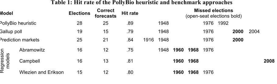
We compared PollyBio’s performance to the predicted two-party vote shares from the final pre-election Gallup poll. The Gallup polling data for the 18 pre-elections from 1936 to 2004 was obtained from the Appendix to Snowberg et al. (2007). For the 2008 election, the final pre-election poll was obtained from www.gallup.com. The results, reported as the hit rate, are shown in Table 1. The hit rate is the proportion of forecasts that correctly determined the election winner. Four times out of the last 19 elections, the final pre-election Gallup poll predicted the wrong candidate to win the election, which yielded a hit rate of 0.79. By comparison, in failing three times out of 28 elections, PollyBio’s hit rate was 0.89.
Table 1: Hit rate of the PollyBio heuristic and benchmark approaches Model Elections Correct
forecasts Hit rate
Missed elections
(open-seat elections bold)
PollyBio heuristic 28 25 .89 1948 1976 1992
Gallup poll 19 15 .79 1948 1976 2000 2004
Prediction markets 25 21 .84 1916 1948 1976 2000
Abramowitz 16 12 .75 1948 1960 1968 1976
Campbell 16 13 .81 1960 1968 2008
Re g re s s io n mo d e ls
Wlezien and Erikson 15 12 .80 1960 1968 1976
PollyBio versus prediction markets
Prediction markets to forecast election outcomes have been already popular in the late 19th century. Rhode and Strumpf (2004) studied historical betting markets that existed for the 15 presidential elections from 1884 through 1940 and found that these markets “did a remarkable job forecasting elections in an era before scientific polling”. In 1988, the Iowa Electronic Market (IEM) was launched as an internet-based futures market in which contracts were traded on the outcome of the presidential election that year. Initially, the IEM provided more accurate election forecasts than traditional opinion polls. In analyzing 964 polls for the five presidential elections from 1988 to 2004, Berg et al. (2008) found that IEM market forecasts were closer to the actual election results 74% of the time. However, this advantage seems to disappear when comparing the market forecasts to a more sophisticated reading of polls. In analyzing data from the same elections, Erikson and Wlezien (2008) found that polls, which had been combined and damped, were more accurate than both the IEM winner-take-all and the vote-share markets.
IEM. (For the three elections from 1964 to 1972, we were unable to obtain prediction market data.) The three datasets were slightly different. While the Wall Street Curb markets and the bookmakers predicted the Electoral College winner, the IEM provided a forecast of the popular vote winner. Nonetheless, each market provided winner-take-all prices. This price can be interpreted as the probability with which the market expects a candidate to win. For example, a market price of $80 indicates an 80% chance of winning. Thus, if the (normalized) price of a candidate exceeded 50%, this candidate was predicted to be the election winner. The results are shown in Table 1. The prediction markets got 21 out of the last 25 elections correct which led to a hit rate of 0.84.
PollyBio versus regression models
Finally, we compared PollyBio’s hit rate to three well-established regression models for which we could obtain out-of-sample forecasts for early elections. Abramowitz (1996) and Campbell (1996) published out-of-sample forecasts from 1948; Wlezien and Erikson’s forecasts were available from 1952 (Wlezien 2001). For the three most recent elections, forecasts were derived from the authors’ respective publications in the elections symposia in PS: Political Science and Politics, 34(1), 37(4), and 41(4). The results are shown in Table 1. In predicting 16 elections,
Abramowitz’s model failed four times, yielding a hit rate of 0.75. Both Campbell (n=16
elections) and Wlezien and Erikson (n=15 elections) missed the correct winner three times, which led to hit rates of 0.81 and 0.80, respectively.
In sum, none of the benchmark approaches achieved a hit rate as high as PollyBio. This performance was achieved even though PollyBio used only information from the respective election year. By comparison, the forecasts from the three regression models relied on historical data from previous elections or were calculated through jackknifing (or cross-validation). This means that the forecasters used N-1 observations from the dataset to calibrate the model and then made a forecast for the one remaining election. Also, note that PollyBio forecasts can be made as soon as the candidates are known; they can even be issued before, conditional on who is expected to run for office. By comparison, the forecasts of the three regression models are issued much later, usually around August and September in the election year. Furthermore, even the final Gallup pre-election polls as well as election-eve prediction market prices were less accurate than PollyBio.
The benefits of biographical information in predicting open-seat elections
Otherwise, they will support the candidate of the other party. Both the models of Abramowitz as well as Wlezien and Erikson use economic growth and presidential approval as predictor
variables; Campbell uses economic growth and measures public support for candidates by
incorporating trial-heat polls. For an overview of the predictor variables used by different models see Jones and Cuzán (2008).
However, in looking at presidential elections as a referendum on the incumbent’s performance, forecasting becomes difficult for open-seat elections without an incumbent in the race. In general, open-seat elections are considered as harder to forecast since voters are expected to vote less retrospectively. Campbell (2008) compared the outcomes of the 13 open-seat elections to the 22 elections with an incumbent in the race that were held between 1868 and 2004. He found that open-seat elections were more often near dead heats than elections with an incumbent running. Also, out of the 11 elections in his sample that were decided in landslide victories, only two were open-seat.
The results in Table 1 support the speculation that the performance of traditional election forecasting models is limited when predicting open-seat elections. All three regression models failed in correctly predicting the winner of the elections in 1960 and 1968 and Campbell’s model also failed in 2008. Each of these elections was an open-seat election. By comparison, as
indicated with the black bars in Figure 1, PollyBio correctly predicted the winner for each of the nine open-seat elections in our sample. The reason might be that PollyBio does not incorporate a measure that relates to the incumbent president’s performance. The results suggest that our model is particularly helpful in predicting the outcome of open-seat elections and, thus, improves on traditional forecasting models.
When biographical information might not be enough: elections with incumbents in the race
PollyBio failed in predicting the correct winner for the three elections in 1948, 1976, and 1992, in each of which an incumbent president was running. A look at the data helps to explain the failure for these three elections. Gerald Ford in 1976 and George Bush in 1992, who were both wrongly predicted to win, had particularly strong biographies. For our set of ‘yes / no’ cues, which did not include relative measures between candidates (like height, intelligence, or attractiveness), Ford and Bush achieved the highest score of all 56 candidates in our sample (together with Theodore Roosevelt in 1904 and William McKinley in 1900). By comparison, Harry Truman, who
achieved the lowest score of all incumbents in the sample. Among all candidates, only three achieved a lower score.
Apparently, while biographical information is helpful to predict open-seat elections, its predictive accuracy seems to decrease if an incumbent president is in the race. The reason appears to be obvious. In relying only on the biographies of candidates, PollyBio is unable to account for situational factors like how the economy is doing or whether the voters approve or disapprove with how the incumbent president is doing his job. Thus, it might be helpful to extend the model by accounting for such factors. We will get back to this in the next section.
Predicting the vote share
Although predicting the correct winner of an election might be the most important criteria to assess the performance of a forecasting method, quantitative models usually provide predictions of the actual vote shares. We tested how well PollyBio forecasts the incumbent candidates’ percentage of the two-party vote for the past 28 elections.
The PollyBio quantitative model
For this, it was necessary to use information from other election years. We used the relative PollyBio score (IPB) of the candidate of the incumbent party as our predictor variable. The IPB is
the percentage of the issues that favored the candidate of the incumbent party. It is defined as:
IPB = [PBIncumbent / (PBIncumbent + PBChallenger)]*100.
We related the IPB to the dependent variable, which was the actual two-party vote share received by the candidate of the incumbent party (V). That is, we used only a single predictor variable to represent all issues. We performed a simple linear regression by relating V to IPB for the period
from 1900 to 2008 and obtained the following vote equation:
PollyBio: V = 20.0 + 0.612 * IPB
Thus, the model predicts that an incumbent would start with 20% of the vote, plus a share depending on the IPB. If the percentage of biographical cues favoring the incumbent went up by
10 percentage points, the incumbent’s vote share would go up by 6.12%. Furthermore, consistent with traditional forecasting models, the model reveals a slight advantage for the incumbent. If both candidates achieve equal index scores (i.e., an IPB score of 50%), the candidate of the
PollyBioA: Accounting for situational factors
In an attempt to account for situational factors, we experimented with adding presidential approval to the model. Presidential approval ratings provide a percentage of how many
respondents approve the way the incumbent president is doing his job and, thus, are an important part of the president’s biography. Introduced by George Gallup in the late 1930s, they were only available for elections from 1940.
For the 12 elections from 1940 to 2008 in which an incumbent was running, we used the
incumbent president’s approval rating from January of the respective election year. For all other elections, we used a dummy value of 50%. We extended the original PollyBio model by adding presidential approval (A) as a second variable to our regression equation (in the following
referred to as PollyBioA). Again, we performed a simple linear regression by relating V to IPB and
PA for the 28 elections from 1900 to 2008 and derived the following vote equation:
PollyBioA: V = 0.166 + 0.589 * IPB + 0.086 * A.
Thus, the model predicts that an incumbent would start with 16.6% of the vote, plus additional shares depending on the IPB and A. If the percentage of biographical cues favoring the incumbent
went up by 10 percentage points, the incumbent’s vote share would go up by 5.89%. Similarly, if the incument president’s approval rating went up by 10 percentage points, his vote share would go up by 0.86%
Accuracy of PollyBio and PollyBioA (jackknifing)
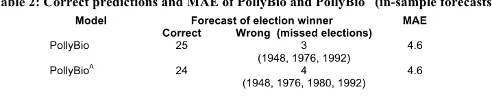
[image:13.612.128.487.561.633.2]Table 4 shows out of sample forecasts of both model variations, calculated through jackknifing. Similar to the heuristic-based approach, PollyBio correctly predicted 25 elections and failed for the elections in 1948, 1976, and 1992. Surprisingly, although PollyBioA yielded a similar mean absolute error (MAE), its accuracy in predicting the winner decreased to 24 correct predictions.
Table 2: Correct predictions and MAE of PollyBio and PollyBioA (in-sample forecasts) Forecast of election winner MAE
Model
Correct Wrong (missed elections)
PollyBio 25 3
(1948, 1976, 1992)
4.6
PollyBioA 24 4
(1948, 1976, 1980, 1992)
4.6
are only available for elections from 1940 and provide no additional information for open-seat elections.
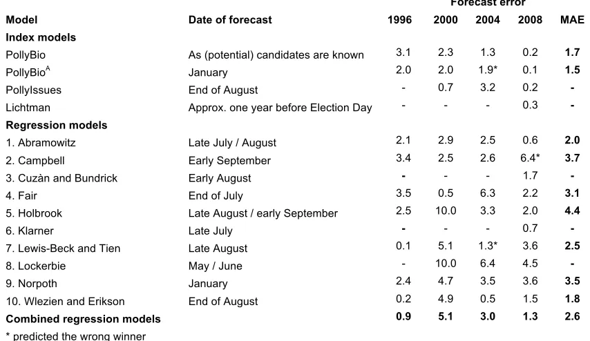
To further examine the relative performance of both model variations, we generated out-of-sample forecasts for the last 4 elections from 1996 to 2008 by successive updating. That is, we only used data from historical elections prior to the respective election year (i.e. we created forecasts for years not included in the estimation sample). The results are shown in Table 3, along with out-of-sample forecasts from two other index models and 10 well-established regression models. For our comparison, we used the forecasts published in American Politics Quarterly
[image:14.612.91.518.346.593.2]24(4) and PS: Political Science and Politics, 34(1), 37(4), and 41(4). The forecasts for Fair’s model were obtained from his website http://fairmodel.econ.yale.edu. The forecasts for Lichtman’s model and PollyIssues were obtained from Lichtman (2008) and Graefe and Armstrong (2008), respectively. For an overview of the predictor variables used in most of the models see Jones and Cuzán (2008).
Table 3: PollyBio and PollyBioA versus other forecasting models: out-of-sample forecasts for 1996 to 2008 Forecast error
Model Date of forecast 1996 2000 2004 2008 MAE
Index models
PollyBio As (potential) candidates are known 3.1 2.3 1.3 0.2 1.7
PollyBioA January 2.0 2.0 1.9* 0.1 1.5
PollyIssues End of August - 0.7 3.2 0.2 -
Lichtman Approx. one year before Election Day - - - 0.3 -
Regression models
1. Abramowitz Late July / August 2.1 2.9 2.5 0.6 2.0
2. Campbell Early September 3.4 2.5 2.6 6.4* 3.7
3. Cuzàn and Bundrick Early August - - - 1.7 -
4. Fair End of July 3.5 0.5 6.3 2.2 3.1
5. Holbrook Late August / early September 2.5 10.0 3.3 2.0 4.4
6. Klarner Late July - - - 0.7 -
7. Lewis-Beck and Tien Late August 0.1 5.1 1.3* 3.6 2.5
8. Lockerbie May / June - 10.0 6.4 4.5 -
9. Norpoth January 2.4 4.7 3.5 3.6 3.5
10. Wlezien and Erikson End of August 0.2 4.9 0.5 1.5 1.8
Combined regression models 0.9 5.1 3.0 1.3 2.6 * predicted the wrong winner
all models for the 2008 election. Recall that this was achieved with a forecast that was issued long before most of the benchmark forecasts were available.
Discussion
Candidates’ biographies incorporate much information about their chances to win elections. Based on a simple heuristic, our PollyBio model was able to correctly predict the winner for 25 out of the last 28 U.S. presidential elections. Furthermore, in using it in combination with linear regression, on average, two variations of our model provided more accurate forecasts of the two-party vote shares than 12 benchmark models for the last four elections. This was achieved by assigning unit weights to biographical information from 49 cues. PollyBioA additionally incorporated presidential approval ratings to account for situational factors.
Unit weighting provided a reasonable starting point, as we did not have prior knowledge about the relative importance of the cues. Furthermore, as with an increasing number of cues the importance of using specific weights generally decreases, PollyBio lend itself to the use of unit weighting. Also, we deliberately did not conduct an ex post analysis to determine the importance of each cue for predicting the outcome. Thus, our model might even include cues that have a negative impact on the outcome. However, since cues were subjectively assessed to be
informative, they might as well have a positive effect when generalizing to new observations. In general, we believe that having all relevant cues in the model improves its robustness and, thus, its predictive accuracy. Furthermore, this approach is fast, inexpensive, and the heuristic-based approach does not require sample size. In addition, we believe that this approach comes close to how most informed voters actually process information. They look over the political resume of the candidates and draw an overall impression using crude (approximately unit) weights.
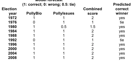
Table 4: Combined forecasts of PollyBio and PollyIssues for the last 10 elections from 1972 to 2008 Model forecast
(1: correct; 0: wrong; 0.5: tie) Election
year PollyBio PollyIssues
Combined score
Predicted correct winner
1972 1 1 2 yes
1976 0 1 1 tie
1980 1 0.5 1.5 yes
1984 1 1 2 yes
1988 1 1 2 yes
1992 0 1 1 tie
1996 1 1 2 yes
2000 1 1 2 yes
2004 1 1 2 yes
2008 1 1 2 yes
PollyBio makes a useful contribution to forecasting accuracy, in particular for forecasting open-seat elections. Following the principle of combining (Armstrong 2001), it appears worthwhile to combine its forecasts with those from other index models that rely on completely different information like the PollyIssues model (Graefe & Armstrong 2008). In applying the index method to predict U.S. presidential elections based on how voters perceive the candidates to deal with the issues facing the country, PollyIssues correctly identified the winner for nine out of the last ten elections, with one tie. Table 4 shows the combined forecasts of the PollyBio and
PollyIssues heuristics for the last 10 elections. For seven elections, the forecasts were in unison in predicting the correct winner, twice the combined forecast would have predicted a tie, and in 1980, the PollyBio forecast correctly resolved PollyIssues’ prediction of a tie. More important, there were no cases in which both forecasts were incorrect. The development of further index models might enhance the accuracy of the combined forecasts and would help creating a knowledge model that incorporates information from various domains. For example, future models could analyze (1) which policies are pursued by candidates and how these are supported by voters (PollyPolicies) or (2) how certain personality traits of candidates are perceived by voters (PollyPersonality).
In combining forecasts from four components (opinion polls, the IEM prediction market, expert judgments, and quantitative models), the PollyVote (www.pollyvote.com) provided highly accurate forecasts for the five U.S. presidential elections from 1992 and 2008 (Graefe et al. 2009). We plan to add a fifth component, index models, to further improve on the accuracy of the PollyVote.
Unfortunately, the simplicity of the index model may be the method’s biggest drawback.
Summarizing evidence from the literature, Hogarth (2006) showed that people exhibit a general resistance to simple solutions. Although there is evidence that simple models can outperform more complicated ones, there is a belief that complex methods are necessary to solve complex problems.
Conclusion
We applied the index method to the 28 U.S. Presidential Elections from 1900 to 2008 and
provided a forecast based on biographic information about candidates. For 25 of the 28 elections, PollyBio correctly predicted the winner. In addition, it provided accurate out-of-sample forecasts for the last 4 elections from 1996 to 2008, outperforming 12 benchmark models.
In using a different method and drawing on different information than traditional election forecasting models, we believe our approach will make a useful contribution to forecasting accuracy, in particular for forecasting open-seat elections. It is simple to use and easy to
understand. Moreover, it can help political parties in nominating candidates running for office.
Acknowledgments
Roy Batchelor, Ray Fair, and Dean K. Simonton provided helpful comments. Andrew Dalzell,
Ishika Das, Max Feldman, Greg Lafata and Martin Yu helped with collecting data.
References
Abramowitz, A. I. (1996). Bill and Al's excellent adventure: Forecasting the 1996 presidential election, American Politics Research, 24, 434-442.
Antonakis, J. & and Dalgas, O. (2009), Predicting Elections: Child’s Play!, Science, 323, 1183.
Armstrong, J. S. (1985). Long-range forecasting: From crystal ball to computer, New York: John Wiley.
Armstrong, J. S. (2001). Combining forecasts. In: J. S. Armstrong (Eds.), Principles of forecasting. A handbook for researchers and practitioners. Norwell; Kluwer Academic Publishers, pp. 417-439.
Armstrong, J. S. & Cuzán, A. G. (2006). Index methods for forecasting: An application to the American Presidential Elections, Foresight, 2006, 10-13.
Berg, J., Nelson, F. & T. A. Rietz (2008). Prediction market accuracy in the long run.
International Journal of Forecasting, 24, 285-300.
Campbell, J. E. (1996). Polls and votes: the trial-heat presidential election forecasting model, certainty, and political campaigns, American Politics Research, 24, 408-443.
Campbell, J. E. (2008). The trial-heat forecast of the 2008 presidential vote: Performance and value considerations in an open-seat election, PS: Political Science & Politics, 41, 697-701.
Cuzán, A. G. & Bundrick, C. M. (2009). Predicting presidential elections with equally-weighted regressors in Fair's Equation and the Fiscal Model. Political Analysis, 17, 2009, 333-340.
Cuzán, A. G. & Heggen, R. J. (1984). A fiscal model of presidential elections in the United States, 1880-1980, Presidential Studies Quarterly, 14, 98-108.
Czerlinski, J., Gigerenzer, G. & Goldstein, D. G. (1999). How good are simple heuristics? In: G. Gigerenzer & Todd, P. M. (Eds.), Simple heuristics that make us smart. Oxford University Press, pp. 97-118.
Dana, J. & Dawes, R. M. (2004). The superiority of simple alternatives to regression for social science predictions, Journal of Educational and Behavioral Statistics, 29, 317-331.
Einhorn, H. J. & Hogarth, R. M. (1975). Unit weighting schemes for decision-making,
Organizational Behavior & Human Performance, 13, 171-192.
Erikson, R. S. & C. Wlezien (2008). Are political markets really superior to polls as election predictors? Public Opinion Quarterly, 72, 190-215.
Fair, R. C. (1978). The effect of economic events on votes for president, Review of Economics and Statistics, 60, 159-173.
Gough, H. G. (1962). Clinical versus statistical prediction in psychology. In: L. Postman (Eds.),
Psychology in the making. New York; Knopf, pp. 526-584.
Graefe, A. & Armstrong, J. S. (2008). Forecasting elections from voters’ perceptions of candidates’ ability to handle issues, Available at
http://www.forecastingprinciples.com/PollyVote/images/articles/index_us.pdf.
Graefe, A., Cuzán, A. G., Jones Jr, R. J. & Armstrong, J. S. (2009). The PollyVote: Combining forecasts to predict U.S. presidential elections, Working Paper, Available from the author.
Hogarth, R. M. (2006). When simple is hard to accept. In: P. M. Todd & Gigerenzer, G. (Eds.),
Ecological rationality: Intelligence in the world (in press). Oxford; Oxford University Press, pp.
Jones, R. J. & Cuzán, A. G. (2008). Forecasting U.S. presidential elections: A brief review,
Foresight, 2008, 29-34.
Lichtman, A. J. (2008). The keys to the white house: An index forecast for 2008, International Journal of Forecasting, 24, 301-309.
Rhode, P. W. & K. S. Strumpf (2004). Historic presidential betting markets, Journal of Economic Perspectives, 18, 127-142.
Simonton, D. K. (1993). Putting the best leaders in the White House: Personality, policy, and performance, Political Psychology, 14, 537-548.
Snowberg, E., Wolfers, J. & E. Zitzewitz (2007). Partisan impacts on the economy: Evidence from prediction markets and close elections, Quarterly Journal of Economics, 122, 807-829.