Contagion of financial crises in sovereign debt markets

Munich Personal RePEc Archive

Contagion of financial crises in sovereign

debt markets

Lizarazo, Sandra

Universidad Carlos III de Madrid

6 February 2009

Online at

https://mpra.ub.uni-muenchen.de/82612/

Contagion of Financial Crises in Sovereign Debt Markets

Sandra Valentina Lizarazo

Universidad Carlos III de Madrid

This version: May 15, 2015 First draft: February 6, 2009

Abstract

This paper develops a DSGE model of sovereign default and contagion for small open economies that have common risk averse international investors. The financial links generated by these investors explain the endogenous determination of credit lim-its, capital flows, and the risk premium in sovereign bond prices. In equilibrium, these variables are a function of both an economy’s own fundamentals and the fundamentals of other economies. The model replicates the Wealth and Portfolio Recomposition channels of contagion, and identifies another channel: the Risk Diversification chan-nel of contagion. Quantitatively, the model is consistent with the contagion of the Argentinean crisis to Uruguay.

JEL Classification: F32; F34; F36; F42

Keywords: Contagion; Sovereign Default Risk; Financial Links; Default; Flight to Quality.

1

Introduction

In the last several decades, the world has witnessed several financial crises that have occurred simultaneously across countries. Examples include the Debt Crisis of 1982, the Mexican Crisis of 1994, the Asian Crises in 1997, the Russian Crisis of 1998, and more recently the 2007-2008 financial crisis and the Euro-debt Crisis in 2011. While the simultaneity of crises could be explained by the occurrence of a common shock to several economies, contagion is another plausible explanation, and the one this paper will focus on. Contagion corresponds to the transmission of a negative income or financial shock from one economy to other economies. The empirical literature that looks at the simultaneity of crisis is quite large, and evidence of contagion in sovereign bond markets is considerable.1

The current paper is concerned with advancing an endogenous theory of contagion of financial crises based on financial links between economies. Countries are linked financially when they have common investors. The emphasis on financial links is strongly supported in the empirical literature.2

The model in this paper studies financial market links across countries in a dy-namic stochastic general equilibrium (DSGE) setting where the stochastic processes of the emerging economies’ bond prices are endogenously determined. The model ex-tends the literature in endogenous sovereign risk in order to consider sovereign bond markets in a multi-country framework.3 _{This type of model allows for an}

endoge-nous determination of the price of one period non-contingent discount bonds as a function of the economy’s default risk. Through the consideration of financial links across economies, the default risk of any economy becomes a function not only of the domestic fundamentals but also a function of the fundamentals of countries which share investors with the domestic country. The model is used to show quantitatively

1_{See for example Valdes (1996), Baig and Goldfajn (1998), Edwards (2000), Baig and Goldfajn}

(2000), Dungey et al.(2002), Jaque (2004), and Ismailescu and Kazemi (2011).

2_{See for example Kaminsky and Reinhart (1998), Van Rijckeghem and Weder (1999), Kaminsky}

and Reinhart (2000), Hernandez and Valdes (2001), Kaminsky et al. (2004), Broner et al. (2006), and Hau and Rey (2008).

3_{Some of the relevant papers considering a single country include Aguiar and Gopinath (2006),}

that contagion can explain co-movements in the price of emerging economy bonds, capital flows, output and consumption beyond the level explained by a country’s own fundamentals.

The theory of contagion in this paper is closely related to the theories of contagion in the more recent papers by Park (2012), and Arellano and Bai (2013). The main differences between the model in this paper and the models in Park (2012), and Arellano and Bai (2013) are the channels of contagion under consideration. This paper analyzes three channels of contagion: the wealth channel of contagion, the portfolio recomposition channel of contagion, and the risk diversification channel of contagion. Under the assumption of decreasing absolute risk aversion (DARA) in the preferences of the investor, these channels can explain contagion in models with two or more countries, and in models for small or large open economies. In contrast, Park (2012) focuses solely on the liquidity channel of contagion: a default by a country in the investor’s portfolio triggers margin calls to the investor that force her to liquidate investments in other countries, and contagion occurs. When more than two countries are considered the liquidity channel of contagion gives the counterintuitive result that the countries with more solid fundamentals are the ones experiencing contagion.

4 _{The two novel and main channels of contagion discussed in Arellano and Bai}

(2013) are the channel of contagion through the effect of a domestic shock in the international interest rate, and the channel of contagion through a strategic collusion between defaulting countries in order to renegotiated debt obligations after a default. These channels work only for the case of “large” open economies, which are able to affect the international interest rate, and have bargaining power in negotiations with the lenders after a default.

Within the present model, the framework is one of a set of small open economies with stochastic endowments. These small open economies have access to an inter-national credit market populated by interinter-national investors. Interinter-national investors are assumed to be risk averse, with preferences that exhibit decreasing absolute risk

4_{Kaminsky and Reinhart (2000) explain the issues of the liquidity channel of contagion. The}

aversion in wealth (DARA). There is a problem of enforcement in the sense that international investors cannot force the small open economies to repay their debts. If any economy defaults, it is temporarily excluded from the world credit market. This context forces international investors to consider the risk of default when choos-ing their portfolio. Any type of reallocation of the international investors portfolio has effects over several countries at the same time. Therefore, the risk of default is endogenously determined by the economy’s own fundamentals, and by the fundamen-tals of other economies: income shocks to an emerging economy generate changes in the risk of default in that economy, and, through financial links, these changes in turn impact other emerging economies. Financial links generate contagion through three channels, the Wealth channel, the Portfolio Recomposition channel, and the

Risk Diversification channel.

(i) The Wealth Channel of Contagion: When an income shock in a country forces that country into default, the shock generates losses for international investors. If the preferences of the investors exhibit DARA, the negative wealth effect of the shock reduces investors’ tolerance for risk. A reduction in tolerance for risk makes investors shift away from risky investments (countries) toward riskless investments (T-Bills). Countries that initially neither default nor face an income shock would face a reduction in the amount of resources available to borrow from, leading to contagion.

(ii) ThePortfolio Recomposition Channel of Contagion: When the risk of de-fault is correlated across countries, an increase in the risk of dede-fault in one coun-try modifies the optimal portfolio of international investors. As investors adjust their portfolios, some countries which did not face an income shock nonetheless face a reduction in the amount of resources available to borrow from, leading to contagion. Other countries, receiving capital inflows, experience flight to quality.

The wealth channel of contagion is analyzed in Kyle and Xiong (2001), Lagunoff and Schreft (2001), and Goldstein and Pauzner (2004). These papers show that if investors’ preferences exhibit DARA, then as a consequence of the reduction on their tolerance toward risk at lower levels of wealth, the optimal response of the investors to financial losses is to reduce their risky investments. The portfolio recomposition channel of contagion is studied in the theoretical papers of Choueri (1999), Schinasi and Smith (1999), Kodres and Pritsker (2002), Broner et al. (2006), and Hau and Rey(2008). Using a partial equilibrium approach where the determination of asset returns is exogenous to the model, these papers highlight the fact that contagion might be successfully explained by standard portfolio theory: in order to reestablish the optimal degree of risk exposure in their portfolio after a negative shock to the return of the assets of some economy, it is optimal for investors to liquidate holdings of assets with expected returns that exhibit some correlation with the expected return of the crisis country.

The results of the current paper are consistent with the empirical evidence regard-ing contagion as a consequence of financial links. First, since investors’ preferences exhibit DARA, they are able to tolerate more default risk when they are wealthier. As a consequence, both capital flows to emerging economies and the equilibrium price of sovereign bonds are increasing functions of investors’ wealth levels. Furthermore, the high correlation between investors’ wealth and emerging economies’ financing condi-tions can account for the simultaneity of crises because a default by any economy is equivalent to a negative wealth shock to the investors. This shock is transmitted to other countries via the wealth channel of contagion.

assets of the economies whose risk did not increase too much. This effect would tend to increase capital flows to some emerging economies. For any country different from the crisis country, if the first effect dominates contagion is observed: the correlation of capital flows across emerging economies is positive. On the other hand, if the second effect dominates, “flight to quality” is observed: emerging economies with robust fundamentals receive capital flows when other countries are affected by financial crises. In practice, whenever the economies fundamentals are sufficiently weak, the effect of the expected negative wealth shock will dominate the substitution effect.

Third, the likelihood of default in equilibrium for any emerging economy is a function also of other emerging economies’ fundamentals. In the numerical simulation in the present paper, for economies with relatively high default probabilities, default is more likely to be an equilibrium outcome when the fundamentals of other economies deteriorate and sovereign spreads are positively correlated.

The quantitative part of the paper studies the case of the contagion of the Argen-tinean crisis to Uruguay and compares the results of this model with the results of a model of endogenous sovereign risk without financial links across economies. These results suggest that the model with financial links is able to endogenously explain the positive correlation between spreads of relatively volatile emerging economies, and the increase in the probability of default of an economy when another economy in the common investors’ portfolio is at the verge of default. At the same time the model delivers reasonable predictions for other real business cycle statistics of the economies under study.

The paper proceeds as follows: Section II develops the model; section III focuses on characterizing contagion; section IV presents the numerical results of the paper; and section V concludes.

2

The Model

Definition 1 The state of the world in the model, S = (s, W), is given by the re-alization of the emerging economies’ fundamentals, s = s1 ×s2 ×. . .×sJ and the representative investor’s asset position or wealth, W ∈ W ≡[W ,∞), W corresponds to the natural debt limit discussed in Aiyagari (1994). In this model, sj = (bj, yj, dj), bj ∈ B ≡[b,∞) is economy j’s asset position where b is endogenously determined in the model, yj ∈ Y is economy j’s endowment, and dj is a variable that describes if economy j is in default or repayment state.

To simplify the notation of the model, in what follows S−j will refer to all the

state variables of the model except for the fundamentals of emerging economyj, that

isS−j = ({sk}J_k=1,k6=j, W). Also, to simplify the notation in what followsS∗′ and S−∗′j

refer to next period state of the model with the variables taking their equilibrium values.

2.1 Sovereign Countries

There are J < ∞ identical small open economies each populated by risk averse households that maximize their discounted expected lifetime utility from consumption

max {cj,t}∞_t=0

Eτ

∞

X

t=0

βtu(cj,t) (1)

where 0< β <1 is the discount factor and cj, t is emerging economyj’s consumption

at time t. The periodic utility of emerging economy j takes the functional form

u(cj) = c1j−γ

1−γ whereγ >0 is the coefficient of relative risk aversion.

In each period, the households of each economy j receive a stochastic stream of consumption goods yj. This income is independently distributed across emerging economies, and its realizations are assumed to have a compact support Y and to follow a Markov process with a transition function f(y′

j | yj). Households in each

economy j also receive a lump-sum transfer Tj from their government.

non-contingent bonds with international investors.5 _{The governments use their access to}

financial markets to smooth the consumption path of the households in their economy.

In the international financial markets the governments borrow or save by buying one period bondsb′

j at price qj(b′j, S). Both the investors and each government ksuch

that k 6= j take as given the price of economy j’s non-contingent discount bonds. In each period, the proceeds of these bonds are rebated back to the households in economy j.

The bonds of any emerging economy j, b′_j, are risky assets because debt con-tracts between the government and the investors are not enforceable. At any time, government j can choose to default on its debt. If the government defaults, all its current debt is erased, and the government is temporarily excluded from international financial markets. Defaulting also entails a direct output cost for country j.

Because international investors are risk averse, the bond prices of the emerging economies,qj(b′j, S) forj = 1, . . . , J, have two components: the price of the expected

losses from default qRN

j (δj(b′j, S)) that corresponds to the price of riskless bonds, qf_{, (hereafter T-Bills) adjusted by the default probability δ}

j(b′j, S), and an “excess”

premium or risk premium ζ_jRA(b′_j, S).

For any emerging economy j, when b′_j ≥ 0, the probability of default for the economy, δj(b′_j, S), is 0. Since the asset is riskless in this case, the risk premium,

ζRA

j (b′j, S), is also 0. Therefore, the price of economyj’s bond is equal to the price of

T-Bills which is qf ₌ 1

1+r, where r is the constant international interest rate. Only

when b′

j ≤0 can δj(b′j, S) andζjRA(b′j, S) be different from 0.

For any economy j, when its government chooses to repay its debts, the resource constraint of the emerging economy is given by

cj =yj−qj(b′_j, S)b′_j +bj. (2)

For the same economy, when the government chooses to default the resource

con-5_{Throughout the paper it is assumed that the governments of the economies are not able to trade}

straint is given by

cj =ydef_j (3)

where y_jdef =h(yj) and h(yj) is an increasing function.

Define V0

j (S) as the value function of the government of economy j that has the

option to default. The government starts the current period with assetsbj and income yj; the other economies that share investors with country j start the current period

with assets bk and income yk for k = 1, . . . , J and k 6= j; all these countries face a representative international investor that has wealth W. The government of any economy j decides whether to default or repay its debts to maximize the households’ welfare subject to market clearing conditions, optimization conditions and the law of motion of S. Each government takes as given the repayment/default decisions of the other governments and the investing decisions of the international investors.6

Given the option of default for country j,V_j0(S) satisfies

V_j0(S) = max {R,D}

V_jR(S), V_jD(S) (4)

given S′ = H(S)

whereV_jR(S) is the value to government j of repaying its debt,V_jD(S) is the value of defaulting in the current period, and His the law of motion ofS which is determined by the income shocks realizations of the emerging economies and the asset holding decisions of the investors and the emerging economies in the investors’ portfolio.

If government j defaults, then the value of default is given by

V_jD(yj, S−j) = u(yjdef) +

β Z

y′

1

. . . Z

y′

J

[θV_j0(0, y′_j, S−j′) + (1−θ)VjD(0, yj′, S−j′)] J Y

h=1

f(yh, y_h′)dy_h′.

whereθ is the probability that a defaulting economy regains access to credit markets.

6_{Through the paper it is assumed that the governments of the economies make their}

If government j repays its debts, then the value of not defaulting is given by

V_jR(S) = max

{b′

j}

(

u(yj−qj(b′_j, S)b′_j +bj) +β Z

y′

1

. . . Z

y′

J

V_j0(S′)

J Y

h=1

f(yh, y′_h)dy_h′ )

.

For the government of emerging country j, the repayment/default decision de-pends on the comparison between the value of repaying its debt, V_jR(S), versus the value of opting for financial autarky, V_jD(y_j′, S−j′). The repayment/default decision

is summarized by the indicator variable dj which takes on a value of 1 when the government repays its debt and 0 when the government does not repay its debt.

For each economy j, conditional onS−j , emerging economyj’s default policy can be characterized by its repayment and default sets:

Definition 2 For given S−j, the default set Dj(bj |S−j) consists of the equilibrium set of yj for which default is optimal when the government’s asset holdings are bj:

Dj(bj |S−j) =yj ∈Yj :VRj (S)≤VjD(yj, S−j) .

The repayment setAj(bj |S−j)is the complement of the default set. It corresponds to the equilibrium set of yj for which repayment is optimal when the government’s asset holdings are bj:

Aj(bj |S−j) =yj ∈Yj :VRj(S)> VjD(yj, S−j) .

Equilibrium default sets,Dj(b′_j |S−j′(S)), are related to equilibrium default

prob-abilities, δj(S′ |S), by the equation

δj(b′_j |S′(S)) = 1−Edj′(b′ |S′(S)) =

Z

Dj(b′_j|S_−j′(S))

f(y_j′ |yj)dy_j′ ×

J Y

k=1,k6=j Z

y′

k

f(y′_k|yk)dy_k′. (5)

In this model, conditional on S−j, the well known results of comparative

First, default sets are shrinking in the economies’ assets (i.e. if bj,1 < bj,2 then

Dj(bj,2 |S−j) ⊆ Dj(bj,1 |S−j) ), and therefore the probability of default δj(b′j, S)

is decreasing inb′_j. Second, the governments of the emerging economies only default when the economies are facing capital outflows, i.e. whenbj−qj b′_j(S), Sb′_j(S)<0. Third, conditional on the persistence of the income process not being too high, the default risk of any economy j is larger for lower levels of income. Since the economic intuition of these results is identical to the intuition in the model of endogenous sovereign default risk with risk neutral investors, it will not be discussed in detail here.

On the other hand, as in models of endogenous sovereign risk and risk averse investors (see for example Lizarazo (2013)), the risk premium ζ_jRA(b′_j, S) is also de-creasing in b′

j. Therefore bond prices qj(b′j, S) are increasing in b′j.

2.2 International Investors

There are a large but finite number of identical competitive investors who will be represented by a representative investor. The representative investor is a risk averse agent whose preferences exhibit DARA. The investor has perfect information regard-ing the income processes of the emergregard-ing economies, and in each period the investor is able to observe the realizations of these incomes.

The representative investor maximizes her discounted expected lifetime utility from consumption

E0

∞

X

t=0

β_Ltv cL_t (6)

where cL is the investor’s consumption and v(cL), her periodic utility, is given by

v(cL_{) =} (cL)

1−γL

1−γL , with γL > 0. The representative investor is endowed with some

initial wealth, W0, at time 0; in each period she receives an exogenous income X.

Because the representative investor is able to commit to honor her debt, she can borrow or lend from industrialized countries (which are not explicitly modeled here) by buying T-Bills at the deterministic risk free world price of qf. The represen-tative investor can also invest in non-contingent bonds of the emerging economies

mentioned in the sub-section on the emerging economies, this price is taken as given by both the investor and the governments of the emerging economies.

On investor’s side, the timing of the decisions within each period is as follows: After the shocks to the economies’ income are realized and the governments of these economies make their repayment/default decisions, the investor realizes her gains/losses and observes her actual wealth for the period, W. W is given by

W = ϑT B +PJ_j=1ϑjdj. After observing W, the investor chooses her next period portfolio allocation, investing in the economies whose governments have paid the debt from the previous period, ϑ′_j, and in T-Bills, ϑT B′. Finally, the representative international investor’s consumption, cL, takes place.

In each period the representative investor faces the budget constraint

cL =X+W −qfϑT B′−

J X

j=1

qjϑ′_jdj. (7)

To simplify the investor’s optimization problem, it is assumed that the investor cannot go short in her investments with emerging economies. Therefore, whenever the governments of the emerging economies are saving, the representative international investor receives these savings and invests them completely in ϑT B′. Therefore, for any economy j,ϑ′_j =−b′_j if the economy is borrowing, and is equal to 0 otherwise.

The law of motion of the representative investor’s wealth is given by

W′ =

J X

j=1

ϑ′_jd′_j +ϑT B′. (8)

Further, the representative investor faces a lower bound on her asset holdings

W < 0 that prevents Ponzi schemes, W′ ≥ W. W corresponds to the “natural” debt limit discussed in Aiyagari (1994). Additionally, the investor’s asset position in bonds of the emerging economy is non-negative, i.e. ϑj ≥0 forj = 1, . . . , J.

the value function, V_L0(S), as follows:

V_L0(S) = max

{ϑ′

j} J j=1, ϑ

T B′

(

v(X+W −qfϑT B′−

J X

j=1

qjϑ′_jdj) +βL Z y′ 1 . . . Z y′ J

V_L0(S′)

J Y

h=1

f(yh, y′_h)dy_h′ )

.

subject to

W′ =

J X

j=1

ϑ′_jd′_j+ϑT B′,

W < W,

S′ = H(S).

Because v(cL_{) satisfies the standard Inada conditions, and X is sufficiently large,} cL > 0 always. Because the representative investor is not credit constrained, when

the government does not default in the current period the solution to the investor’s optimization problem can be characterized by the following first order conditions:

ForϑT B′ : qfvcL cL

=βL Z y′ 1 . . . Z y′ J h vcL

cL′i

J Y

h=1

f(yh, y′_h)dy_h′. (9a)

For ϑ′_j : qjvcL cL=βL

Z y′ 1 . . . Z y′ J h vcL

cL′ dj′i J Y

h=1

f(yh, y′_h)dy_h′. (9b)

The set ofJ equations (9) determine the allocation of the representative investor’s re-sources to each one of theJ emerging countries. It is possible to manipulate equations (9) to get

qj = βL Z y′ 1 . . . Z y′ J

vcL cL

′

dj′

vcL(cL)

J Y

h=1

f(yh, yh′)dyh′.

= βL

CovvcL cL

′

, dj′

vcL(cL)

+qRN_j .

= ζ_jRA+q_jRN. (10)

qRN_j , compensates investors for the expected loss from default. The second compo-nent, ζ_jRA, corresponds to the risk premium that economy j’s bonds must carry in order to induce risk averse investors to hold them. The main determinant of the “excess” risk premium ζ_jRA is the covariance term in equation (10). This covariance term is non-positive: Covv_cL cL

′

, dj′

≤0.7

Because cL is a function of W, γL, and the investor’s investments in other economies, it is possible to see from equation (10), that qj for j = 1,· · · , J are also a function of those variables. Therefore, in this model, conditional on S−j, the

comparative statics results of Lizarazo (2013) follow:

(i) For any state of the world,S, as the risk aversion of the international investor in-creases, the governments’ incentives to default increase: As discussed in Lizarazo (2013), γL _{is an important determinant of the emerging economies’ access to}

credit markets and their risk of default. The more risk averse are international investors, the higher is the default risk and the tighter are the endogenous credit constraints faced by all emerging economies. This characteristic of the model is consistent with empirical findings which characterize the role of investor’s risk aversion in the determination of country risk and sovereign yield.8

(ii) Default sets are shrinking in the assets of the representative investor. For all W1 < W2, if default is optimal for bj in some states yj given W2, then

default will be optimal for bj for the same states yj given W1 and

there-fore Djbj |W2,{sk}J_k=1,k6=j ⊆ Djbj |W1,{sk}J_k=1,k6=j: Also as in Lizarazo

(2013), for the present model, other things given the higher isW, the smaller is

7_Forb′

j withδj= 0 orδj = 1, Cov

h

v_cL

cL′

, dj′

i

= 0, andqj =qf or qj = 0 respectively. If

0< δj<1, then for the states of the word next period in which governmentj repays

W′_|d

j′=1

=

ϑj′+PJ_k=1,k6=jϑk

′

dk′+ϑT B′; and for the states in which the governmentj defaultsW′ |dj′=0

=

PJ

k=1,k6=jϑk′dk′ +ϑT B′. Because

W′_|d

j′=1

> W′_|d

j′=0

then hcL′

|dj′=1

i

> hcL′

|dj′=0

i and

by concavity of v(·), hvcL

cL′|dj′=1

i

<hvcL

cL′|dj′=0

i

. As a consequence, for bj′ with more

dj′ = 1, vcL

cL′

is lower. Clearly for this caseCovhvcL

cL′

, dj′

i

<0.

8_{See, for example, Arora and Cerisola (2001), FitzGerald and Krolzig (2003), Ferruci et al.}

the default risk of any economy in the investor’s portfolio, and hence the more relaxed is the economy’s endogenous credit constraint. Several empirical papers are consistent with this characteristic of the model.9 _{This characteristic of the}

model is also consistent with the evidence regarding financial contagion across countries who share investors.10

In comparison with the previous literature on endogenous sovereign default and risk averse international investors, in the current model there is a novel issue: hav-ing investments in several emerghav-ing economies allows the investors to diversify the sovereign risk of any specific economy. In the next subsection, this new issue is briefly discussed.

2.2.1 Risk Diversification

In the current multi-country model, risk diversification is a novel dimension in which the risk aversion on the side of the investors has an important impact on the access to credit for the emerging economies. Risk diversification facilitates the investor’s consumption smoothing; therefore it increases the expected marginal benefit of con-sumption of risky investments (sovereign bonds in the context of this model), and reduces the need for self-insurance (T-Bills in this model).

Risk diversification increases in the model when the investors have access to in-vestments in more emerging economies.11 _{That is, if N is the number of emerging}

economies in the investor’s portfolio and N is relatively small, if the investor can invest in N = N2 countries instead of N = N1 countries with N2 > N1, then the investor’s portfolio is more diversified, and the expected marginal benefit in terms of consumption of a risky portfolio is larger. As a consequence, better access to

9_{See, for example, FitzGerald and Krolzig (2003), Mody and Taylor (2003), Ferruci et al. (2004),}

Gonzales and Levy (2006), and Longstaff et al. (2008). These papers establish that proxies of international investors’ wealth are important factors in the determination of sovereign bond spreads for emerging economies.

10_{See, for example, Kaminsky and Reinhart (1998), Van Rijckeghem and Weder (1999), Kaminsky}

and Reinhart (2000), Hernandez and Valdes (2001), Kaminsky et al. (2004), Broner et al. (2006), and Hau and Rey (2008).

11_{Access to more opportunities for investment helps to diversify the risk of the portfolio only if}

risk diversification allows the investor to better tolerate risk: more opportunities for risk diversification imply more willingness to take sovereign risk by international in-vestors.12 _{Therefore the amount of W that is invested in risky bonds is larger when}

the representative investor has access to a larger number of risky sovereign bonds.

However, when N is relatively large, the effect of having access to investment opportunities in new sovereign bonds is very small or nil. From the investor’s point view, havingN possible investment opportunities generates 2N _{possible states in the}

following period, each with a relatively small individual likelihood of occurrence. This small probability of the individual states facilitates consumption smoothing.

How small N needs to be for the gains from risk diversification to be significant depends mainly on two factors:

(i) The investors’ borrowing limit W : This borrowing limit, which depends on

X and r, determines the maximum total amount of resources that the investor can invest. The larger this borrowing limit is, the smaller is the investors’ opportunity cost of investing in any new risky asset.

(ii) The riskiness of individual sovereign bonds: If the individual investments avail-able to the investors are more risky, there is a higher value of having access to additional sovereign bonds; these additional sovereign bonds make

diversifica-12_{By comparing the RHS of equation (9a) for the case in which the investors can invest only in} one emerging economy (i.e., N = 1) to the case in which the investors can invest in two different emerging economies (i.e.,N = 2), we can see the effect of better opportunities for risk diversification on the need of the investor for self insurance (i.e., investing in safe assets as T-Bills). From the point of view of the investors, whenN = 1 there are only two states of the world in the next period: a state with high consumption that occurs when economy 1 pays back and that has a probability (1−δ1), and a state of low consumption that occurs when economy 1 defaults and that has a probabilityδ1. In contrast, whenN= 2 there are four possible states: a state of high consumption that occurs when the emerging economies pay back and that has a probability (1−δ1)(1−δ2), a state of moderate consumption that occurs when emerging economy 1 pays back and emerging economy 2 defaults and that has a probability (1−δ1)δ2, another state of moderate consumption that occurs when emerging economy 1 defaults and emerging economy 2 pays and that has a probabilityδ1(1−δ2), and a state of low consumption that has a probabilityδ1δ2. If in both scenarios the investors were to invest the same total amount of resources in sovereign bonds, it is clear that whenN = 2 the extreme states of the world - very high or very low consumption - are not as likely as whenN = 1. Therefore, given the concavity ofv(cL), the marginal expected benefit of the investment in T-Bills would be smaller

(i.e.,EhvcL(cL ′

|N = 2)i< EhvcL(cL ′

tion more feasible.

The discussion of international investors illustrates three factors which have an effect on the determination ofqj: investors’ wealth, the fundamentals of other

emerg-ing economies in the investors’ portfolio, and the number of those economies in the investors’ portfolio. Therefore it should be clear that sovereign bond prices across economies that share investors are jointly determined and must be correlated. The discussion of this correlation will be postponed until the section on the characteriza-tion of contagion channels.

2.3 Equilibrium

Let BB and BW be the Borel sigma algebras of B and W, and P(Y) the power set of Y. Let ΣS be the sigma algebra on S,M= (S,ΣS) the corresponding measurable

space, and M the set of all probability measures on M. Let H : M → M be the aggregate law of motion, therefore S′ =H(S).

Definition 3 The recursive equilibrium for the model is defined as a set of policy functions for (i) the emerging economies’ consumption {cj(S)}J_j=1, (ii) the govern-ments’ asset holdings b′_j(S) _j=1J , (iii) the governments’ default decisions {dj(S)}J_j=1

and the associated default sets Dj(bj | S−j), (iv) the representative investor’s

con-sumption cL_{(S), (v) the representative investor’s holdings of emerging economies’} bonds θ′

j(S) J

j=1, (vi) the representative investor’s holdings of T-Bills θ

T B′_{(S), and}

(vii) the emerging economies’ bond price functions qj(S, b′j) J

j=1, such that:

(i) Taking as given the representative investor’s policies and the bond price func-tions qj(S, b′_j) J_j=1, the emerging economies’ consumption {cj(S)}J_j=1 satis-fies the economies’ resource constraints. Additionally, the policy functions

b′

j(S) J

j=1, {dj(S)}

J

j=1 and default sets Dj(bj | S−j) satisfy the optimization problem of the governments of the emerging economies.

(ii) Taking as given the governments’ policies and the bond price functions

qj(S, b′j) J

j=1, the representative investor’s consumptionc

L_{(s)satisfies her}

bud-get constraint. Also, the representative investor’s policy functions ϑ′_j(S) J

and ϑT B′(S) satisfy her optimization problem and the law of motion of her wealth.

(iii) Bond prices reflect the governments’ probabilities of default and the risk premi-ums demanded by the representative international investor. These prices clear the market for all the emerging economies’ bonds:

bj ′(S) = −ϑj ′(S) if bj ′(S)<0 (11a)

0 = −ϑj ′(S) if bj ′(s)≥0. (11b)

(iv) The aggregate law of motion H is generated by an exogenous multivariate inde-pendently distributed Markov process with a transition functionf(y_j′ |yj) J_j=1,

and the policy functions b′

j J

j=1, W

′_.

(a) Define the transition function Q_S,{y

j}Jj=1,{yj′} J j=1

:S×ΣS →[0,1] by13

Q

S,{yj}Jj=1,{y′j} J j=1

(S,ΣS) = ( R

y′

1. . . R

y′

J

QJ

j=1f(yj, yj′)dyj′ for S ∈ΣS

0 otherwise

for all ({yj}J_j=1,

b′_j J

j=1, W)∈S and all (Y

J_{, B}J_,W)∈Σ

S.

(b) Hence

S′ =H(S) =

Z

Q_S,{y

j}J_j=1,{y′_j} J j=1

(S,ΣS)S J Y

j=1

(dbj×dyj)×dW !

3

Contagion

From equation (10) it is evident that in this model the bond prices of economy j

depend on the income realizations of other emerging economies and the associated

13_{In this context Q}

S,{yj}Jj=1,{y′j} J j=1

(S,ΣS) is the probability that economies j = 1, . . . , J with

current assets{bj}J_j=1and income{yj}J_j=1end up with assets

b′_j J

j=1and income

y_j′ J

repayment/default decisions of those countries. Hence, considering a crisis in some foreign emerging economy k as a shock that changes the expected repayment/default decisions of the government of country k, and therefore δk and qk, a crisis in the emerging economy k has three effects over the optimal investor’s portfolio allocation to other emerging economies:

• A wealth effect: Wealth Channel of Contagion

• A substitution effect: The Recomposition Channel of Contagion

• A diversification effect: The Risk Diversification Channel of Contagion

In what follows, mainly for expositional purposes, these three effects are charac-terized as if they operatedseparately. In reality, they interact and sometimes reinforce or modify each other. More specifically, for the discussion of the wealth channel of contagion and the recomposition channel of contagion it will be initially assumed that a default by economyk does not imply a reduction in the diversification opportunities of the investor: This would be the case if once a country defaults it is replaced in the investors portfolio by an identical country with a clean default record. This assump-tion of replacement of the defaulting economy after a default will be eliminated in order to study the Risk Diversification channel of contagion.

3.1 Wealth Channel of Contagion

First, the crisis in countrykhas a negative current or expected wealth effect. Because the investor’s preferences exhibit DARA, she would move away from risky emerging economies’ assets towards safer assets; this effect corresponds to theWealth Channel of Contagion.

Proposition 1 There is a wealth channel of contagion. Because in this model default sets are shrinking in W then if economy k in the investor’s portfolio defaults, then for economyj, which is also in the investor’s portfolio, incentives to default increase.

Proof. See appendix.

because default sets are shrinking in the assets of the representative investor—i.e., the probability of default of any emerging economy is lower when the representative investor is wealthier—the probability of default for other economies in the investors’ portfolio increases as a consequence of the default by economy k.

3.2 The Recomposition Channel of Contagion

Second, the crisis in country k generates substitution between different risky emerg-ing economy assets in the investor’s portfolio. The substitution effect of the crisis corresponds to the Portfolio Recomposition Channel of Contagion.

This channel operates because the increase in δk in this period has two effects on

the portfolio allocation of the representative investor:

(i) The increase in δk reduces the expected wealth of the investor in the following period thereby reducing the investor’s tolerance for risk. This reduction in risk tolerance induces a reduction of the bonds holdings of all risky countries. This effect would imply a contagion of the crisis in country k to country j.14

(ii) The increase in δk increases the marginal expected benefit of all other risky

14_{This effect can be seen by inspection of equation (9a). Other things given, an increase in δ}

k

increases the RHS of equation (9a). For example, in a two-country model, the RHS of equation (9a) is given by:

EhvcL(cL ′

)i =

(1−δj)(1−δk)

h

vcL(cL ′

| d′_j = 1, d′_k = 1)i + (1−δj)δk

h

vcL(cL ′

|d′_j = 1, d′_k = 0)i + δj(1−δk)

h

vcL(cL ′

|d′_j = 0, d′_k= 1)i + δjδk

h

vcL(cL ′

|d′_j= 0, d′_k = 0)i.

All other things equal, an increase inδk has the following effect in the RHS of equation (9a):

∂EhvcL(cL ′

)i

∂δk

= (1−δj)

nh

vcL(cL ′

|d′_j= 1, d′_k= 0)i−hvcL(cL ′

|d′_j= 1, d′_k= 1)io + δj

nh

vcL(cL ′

|d′_j= 0, d′_k= 0)i−hvcL(cL ′

|d′_j = 0, d′_k= 1)io.

The concavity of the investor’s utility function ensures that the two terms in the braces are positive

and therefore ∂E

h v_cL(cL′

)i

∂δk >0. This result implies that the representative investor will optimally

investments. This change induces an increase of the investor’s bonds holdings of all risky countries. This effect would imply flight to quality towards country

j as a consequence of the crisis in country k.15

Since there are two opposing effects at work, it is not possible to unambigu-ously characterize the operation of the portfolio recomposition channel theoretically. However it is clear that the second effect would be stronger for countries for which

∂Ehv_cL(cL′_)d′

j

i

∂δk is relatively large. This would be the case whenever the weights given

to the states of the world in which country j pays its debts increase more after an increase in δk. Using the case of a two-country model for illustrative purposes, it is

possible to show that for that case ∂

2_Eh

v_cL(cL′_)d′

j

i

∂δk∂δj < 0.

16 _{Therefore for the case of a}

two country model the substitution effect of an increase in δk is larger for countries with a small probability of default δj.

The intuition derived from the two-country model seems to suggest that whenever

δk increases, countries with weak fundamentals, which are reflected in high default

probabilities, experience contagion; countries with solid fundamentals, which are

re-15_{This effect can be seen by inspection of equation (9b) for economyj. Other things equal, an} increase in δk increases the RHS of equation (9b) for economy j. For example in a two-country

model the RHS of equation (9b) is given by:

EhvcL(cL ′

)d_j′i = (1−δj)(1−δk)

h

vcL(cL ′

|d′_j = 1, d′_k= 1)i + (1−δj)δk

h

vcL(cL ′

|d′_j = 1, d′_k = 0)i.

All other things equal, an increase inδk has the following effect in the RHS of equation (9b):

∂E

h

vcL(cL ′

)d′_j

i

∂δk

= (1−δj)

nh

vcL(cL ′

|d′_j= 1, d′_k= 0)i−hvcL(cL ′

|d′_j = 1, d′_k= 1)io.

The concavity of the investor’s utility function ensures that the term in the braces is positive and

therefore ∂E

h v_cL(cL′

)d′ j

i

∂δk > 0. Therefore the representative investor will optimally choose to have

larger holdings of countryj sovereign bonds whenδk increases. Clearly this result implies a

substi-tution of countrykbonds for bonds of the other risky economies. 16_{For the case of two countries}

∂2EhvcL(cL ′

)d′_ji ∂δk∂δj

=−(1−δj)

∂EhvcL(cL ′

)d′_ji ∂δk

flected in low default probabilities, experience flight to quality.17

The intuition behind the portfolio recomposition channel can be framed in the context of the previous literature: In a partial equilibrium model of contagion, Kodres and Pritsker (1998) identified the extent of the impact of the shock in one asset over another asset. They find that the impact depends on the degree of correlation between the returns of those two assets. In the context of the current model, this result implies that the impact of a shock in economyk over a particular economyj depends on the strength of the positive correlation between qk and qj.

Quantitatively, the current model exhibits the following property: If the positive correlation between qk and qj is low (i.e., probabilities of default are quite

differ-ent), then the positive substitution effect of the crisis in country k might dominate its negative wealth effect. In this case there is flight to quality. This outcome is observed when the other economies in the investor’s portfolio have relatively sound fundamentals. On the other hand, when the positive correlation between qk and

qj is large (probabilities of default are similar), the negative expected wealth effect dominates. In this case contagion is observed due to portfolio recomposition. This outcome is observed if the other economies in the investor’s portfolio have relatively weak fundamentals.

3.3 The Risk Diversification Channel of Contagion

Third, given the exclusion from credit markets of any defaulting economy and the no-replacement in the investor’s portfolio of that economy by an identical country with a clear default record, default by country k reduces the investor’s opportunities for risk diversification; therefore default by country k increases the investor’s need for self-insurance. On the other hand, default by country k also increases the relative importance of any other risky bond as an available mean to the investor for risk diversification.

17_{Kaminsky, Lyons, and Schmukler (2004) identify flight to quality in the following cases: during}

In order to understand comparative static effects of risk diversification on the investor’s asset holdings of emerging economies bonds ϑj and the interaction of risk diversification with the other contagion channels, we focus on the equations (9) taking

qj and default probabilities δj as given, and assuming that ex-ante all economies are identical.

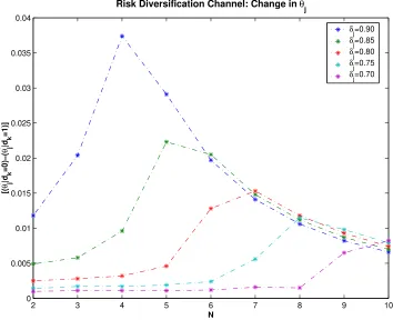
Figure 1 shows the effect of the risk diversification channel on the increase in the investor’s asset holdings of economyj’s bonds when economykdefaults. This increase is plotted as a function of the number of countries N in the investor’s portfolio and for five different levels of δj.18 _{As can be seen in Figure 1, if risk diversification were}

the only channel of contagion in the model—i.e., if the only cost for the investors of economy k’s default is the reduction in the number of countries in their portfolio— then, in response to the default by emerging economy k, flight to quality would be observed.

Since the cost of a default for the investors goes beyond the reduction in their opportunities for risk diversification, the following sub-section looks at the interaction of the wealth channel of contagion and the risk diversification channel of contagion.

3.4 Interaction Between The Wealth and The Risk Diversification

Chan-nels of Contagion

When economy k defaults, two opposing forces come into play: the wealth channel of contagion and the risk diversification channel of contagion. Which of these forces dominates would determine the net effect that a default by an economy k has over any other economy j in the investor’s portfolio.

In this subsection, taking qj and δj as given and assuming that ex-ante all

economies are identical, static comparative analysis of equations (9) shows that the wealth channel of contagion dominates whenever N is small, or whenever the de-faulting economy’s debt with the investors is high.19 _{Additionally, the stronger is}

18_{The increase in the investor’s asset holdings of sovereign bonds is measured as a proportion of}

the mean income level of the emerging economies.

19_{If N is small the investors do not have many opportunities for risk diversification and as a} consequence their exposure to the individual economies is high. If the debt of economyk(θk =−bk)

2 3 4 5 6 7 8 9 10 0

0.005 0.01 0.015 0.02 0.025 0.03 0.035 0.04

Risk Diversification Channel: Change in θ

j

′

N

[(

θ j

′|d k

=0)−(

θ j

′|d k

=1)]

δ_j=0.90 δ_j=0.85 δ_j=0.80 δ_j=0.75 δ_j=0.70

Figure 1: The Risk Diversification Channel of Contagion.

the crisis—i.e. the larger the number of countries that are initially defaulting—the more likely it is that negative contagion towards economy j would be observed after a default by economy k. Finally, the riskier is the average emerging economy in the investor’s portfolio (measuring the risk of the economies by their probability of de-fault), the more likely it is to observe negative contagion to economy j after a default by economy k.

The magnitude of the shock to the wealth of the investors of a default by country

k is given by −bk. From previous models of endogenous sovereign risk, it is known

that in order for an economy to find it optimal to default it must be the case that

bk−qk(b′k, S)b′k<0, i.e., the economy is experiencing capital outflows at the moment

2 3 4 5 6 7 8 9 10 −0.1

−0.08 −0.06 −0.04 −0.02 0 0.02 0.04

Interaction R−D & W Channels: Change in θ

j

′

N

[(

θ j

′|d k

=0)−(

θ j

′|d k

=1)]

θ_k,min

θ_k,med

θ_k,max

(N−1)θ k,min (N−1)θ

k,med (N−1)θ

k,max

Figure 2: Interaction of the Wealth and Risk Diversification Channels of Contagion.

observed for bonds of economy k if the economy repays its debts in this period.20

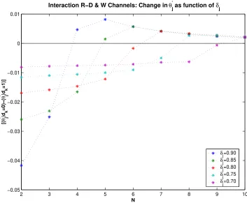
Figure 2 shows the effect of the interaction of the wealth and the risk diversification channels of contagion. Figure 2 shows the increase in the investor’s asset holdings of emerging economy j’s bonds when countryk defaults, as a function of N, for a given

δj, and three different levels of debt of country k.

From Figure 2 it can be seen that after a default by one economy in the investors’ portfolio the net effect on the other economies in the investors’ portfolio would depend on N: for small N (N ≤ 4) the wealth effect dominates the effect of the change in the opportunities for risk diversification. In this case, after a default by economy k, negative contagion to the other economies in the investors’ portfolio is observed. For intermediate values of N (N = 5) the net effect would be negative contagion only

20_Becauseb

if the wealth shock is large enough, i.e. if the debt level of the defaulting economy is sufficiently large. Finally for larger N (N ≥ 6), after a default by country k, the effect of the change in the opportunities for risk diversification cancels out the wealth effect. In this case flight to quality is observed.

The intuition is as follows for the relationship between the net effect of a default by economy k and the size of N: When N is large the investors do not need to hold T-Bills to self-insure; they hold all their wealth in risky bonds. In this case investors have the maximum possible total exposure to risky sovereign bonds but their exposure to individual countries is small. As a consequence of the small exposure to countryk, the default by this country has a small wealth shock; and since after the default the number of opportunities for risk diversification, N −1, is still large, there is no need for the investors to increase their holdings of T-Bills in order to self- insure. In this case investors substitute away from country k’s bonds into the other risky bonds. On the other hand, when N is small, investors need to hold T-Bills to self insure against the countries’ sovereign risk. Additionally the exposure to each individual country in the portfolio is relatively large. Therefore, when country k defaults, the resulting wealth shock is large. Investors substitute away from country k’s bonds into T-Bills.

Figure 2 also shows the interaction of the wealth channel of contagion and the risk diversification channel of contagion for the three different levels of debt for the defaulting countries after a massive default involving N −1 countries (i.e., only one country in the investors’ portfolio does not default initially).

From the comparison between the effect of one country’s default versus a massive default by N−1 countries, it is possible to conclude that the magnitude of the crisis matters to determine if negative contagion or flight to quality is observed after a sovereign crisis: When there is a wide-spread crisis involving several countries, there is a higher likelihood of observing negative contagion instead of flight to quality.

Figure 3 shows the change in the investor’s asset holdings of sovereign bonds of economy j when economy k defaults as a function of N, for a given bk and different

values ofδj. Figure 3 illustrates that other things given, for a riskier set of individual

2 3 4 5 6 7 8 9 10 −0.05

−0.04 −0.03 −0.02 −0.01 0 0.01

Interaction R−D & W Channels: Change in θ

j

′ _{as function of δ}

j

N

[(

θ j

′|d k

=0)−(

θ j

′|d k

=1)]

δ_j=0.90 δ_j=0.85 δ_j=0.80 δ_j=0.75 δ_j=0.70

Figure 3: Wealth and Risk Diversification Channels of Contagion: Portfolio Average Risk.

In terms of the net effect of a default by country k on the other countries in the investor’s portfolio, the findings presented here are in line with recommended safe investment practices: investors are better off when they have small exposure to in-dividual investments, and as much as possible risk diversification of their portfolio. According to the current model, these recommended investment practices make neg-ative contagion less likely to occur, but at the cost of limiting credit flows to the individual economies not only during bad times but also during good times.

3.5 Summary of the Main Findings about Contagion Channels

To summarize the channels of contagion in the current model, the main findings are as follows:

of a default by this country over the other economies in the investor’s portfolio.

• The weaker are the fundamentals of a country, the more likely it is after a default by another country that the weak country faces contagion.

• The more diversified is the investor’s portfolio, the less likely it is that negative contagion occurs after an economy defaults.

4

Quantitative Analysis

The simulation of the model in this paper looks at the Argentinean default of 2001 and its contagion to Uruguay. This case was chosen over the Tequila Crisis or the Russian Default for several reasons:

• The current model focuses on the case of countries that share investors. This assumption disqualifies to a large extent analysis of the contagion of the Russian Default.21

• In the case of the Tequila crisis, there was no actual default, making it hard to see such a case as a straightforward application of the model in this paper.

• The assumption in the model of identical countries except for the actual re-alizations of their endowments seems to better suit the case of Argentina and Uruguay than the cases of the Tequila Crisis or the Russian Default.22

21_{Despite the large impact of the Russian Default on Latin American countries, these countries}

do not seem to share investors with Russia: International investors seem to specialize in specific geographical areas, i.e. some of them focus on Latin America, others in Asia, and some others in the so called economies in transition.

22_{While the estimated process for Argentina and Uruguay are relatively similar, the estimated}

process for Russia and Brazil are quite different and the same is true for the process of Mexico, Brazil, and Argentina:

• Finally, there is a large literature on endogenous sovereign default that looks at the case of the Argentinean default allowing for an easier comparison of the results in this paper with the results of previous models of endogenous sovereign default.

A possible argument against the choice of the Argentinean crisis would be that Argentina and Uruguay share many other links, such as trade, geographical region, similar cultural background, etc., and these links could have a role in explaining the transmission of the crisis. However, as noted in the introduction, the previous empirical literature in contagion has identified financial links as the main channel of transmission of crises.

The aim of this section then is to show quantitatively that even in the absence of additional links across countries, financial links can explain and replicate the follow-ing two observed dynamics of sovereign yield spreads and capital flows to emergfollow-ing economies:

(i) Capital flows and domestic interest rates across emerging economies are posi-tively correlated.

(ii) Default is more likely to be observed when the fundamentals of other emerging economies deteriorate.

4.1 Contagion of the Argentinean Default of 2001

During 2001 Argentina faced one of the worst economic crises of its history. The crisis forced the country to default on US$100 billion external government debt (which cor-responded to nearly 37% of GDP) by the end of 2001, and had strong real effects that extended into 2002: according to estimates from the IMF, during 2001 Argentina’s GDP fell by 4.4% and during 2002 it fell by an additional 10.9%.

Table 1: Contagion: Parameter Values

Parameter Value

Std. Dev. Emerging Economy’s Incomestd[y] 0.025 Autocorr. Emerging Economy’s Income Process 0.945

Emerging Economy’s Discount Factorβ 0.953

Emerging Economy’s Risk Aversionγ 2

Probability of re-entryτ 0.282

Critical level of output for asymmetrical output cost yˆ= 0.969E(y)

Representative investor’s IncomeX 0.01

Representative Investor’s Discount FactorβL _0.98

Representative investor’s Risk AversionγL 2

Risk Free Interest Raterf ₌ 1

qf 0.017

was a significant increase in the public debt to GDP ratio in Uruguay, reaching a level of 52%. According to the estimates of the IMF, during 2001 Uruguay’s GDP fell by 3.5%, and during 2002 Uruguay’s GDP fell by an additional 7.1%.

The fall in GDP in 2002 was due mainly to problems in Uruguay’s financial sector which had strong financial links to Argentina. In early 2002, following the Argentina’s default, Uruguay’s financial sector experienced large dollar deposit outflows (these outflows exceeded US$100 million per day in the month of July 2002), as it faced a rapid decline in its international reserves. Uruguay’s international reserves fell from 3 billion dollars at the end of 2001 to 650 million by August 2002. During 2002, Uruguay’s debt was downgraded by investment rating agencies signaling the credit risk involved in Uruguay’s external debt.

4.1.1 Simulation

Given the assumption of the model of identical economies that only differ in the real-izations of their endowments, and in order to facilitate comparison with the previous literature on the subject, the parameters considered for the simulation are chosen to replicate the features of the Argentinean economy, and are taken from the calibra-tion for this economy in Arellano (2008). The parameters related to internacalibra-tional investors are taken from Lizarazo (2013) which presents a quantitative model with endogenous sovereign risk and risk averse international investors whose preferences exhibit DARA for the case of the Argentinean default.

coeffi-cient of risk aversion of the economy is 2, a standard value considered in the business cycle literature. The free interest rate is set to 1.7%, to match the quarterly US interest rate of a bond with a maturity of 5 years during the period under study. GDP is assumed to follow a log-normal AR(1) processlog(yt) =ρlog(yt−1) +εy with E[εy_{] = 0 and E[ε}y2_{] = σ}2

y. The values estimated for the Argentinean economy are ρ= 0.945 and σy = 0.025. Following a default there is an asymmetrical function for

the output loss as follows:

φ(y) =

( b

y if y >y_b y if y≤_by

)

(12)

with _by = 0.969E(y) which in Arellano (2008) targets a value of 5.53% for the aver-age debt service to GDP ratio. The probability of re-entry to credit markets after defaulting is set at 0.282, which is consistent with the empirical evidence regarding the exclusion from credit markets of defaulting countries (see Gelos et al. (2011)); in Arellano (2008) this value targets a volatility of 1.75 for the trade balance. The discount factor is set at 0.953 which in Arellano (2008) targets an annual default probability of 3%.

The parameters for the international investors are as follows: the representative investor’s discount factor is set to 0.98. As in Lizarazo (2013), if there were no uncertainty, the discount factor of the investors would pin-down the international risk free interest rate (i.e., β_qLf = 1); however, with uncertainty, in order to have a

well defined distribution for the investor’s assets, it is necessary that the discount factor satisfies β_qLf < 1. The value of βL = 0.98 is the highest value in the range

commonly used in business cycle studies of industrialized countries such that for an international interest rate of 1.7% the asset distribution of the investors is well defined. The representative investor’s coefficient of risk aversion is set at 2; this value is chosen to generate a mean spread for model that is as close as possible to the mean spread in Argentina for the period of study, which corresponds to 12.67%.23 _{The representative}

23_{Lizarazo (2013) also considers a value of 5 forγ}L _{which helps to attain a better match for the}

level of the spreads and their volatility, however this larger value forγL_{has important costs in terms}

investor receives a deterministic income ofX = 1% of the emerging economy’s mean income in each period. As in Lizarazo (2013), this parameter is included to preclude the investors from not investing in the emerging economy in order to avoid a negative consumption level in the case of default. Therefore, the strategy for choosing X is to give it as little importance as possible by choosing a value that is close to 0 but that still allows for interior solutions regarding the investor’s investments in the emerging economy’s bonds.24

The model is simulated for two economies that are labeled as (A) and (U) respec-tively. For each economy the endowment shock is discretized into a 9 state Markov chain and the asset position of the economy is approximated by a 75 point grid. The investor’s wealth level is approximated using a 10 point grid, over which the solution to the investor’s problem is linearly interpolated. The business cycles statistics of the model are derived as follows: The model is simulated for 20,000 periods. From these 20,000 periods, sub-samples that have economy A staying in the credit market for 60 periods before going into a default are taken to compute the business cycles statistics of the two economies. This process is repeated 5,000 times, and the cycle statistics are the average of the statistics derived from each of these repetitions.

4.1.2 Results

Table 2 describes the relevant business cycle statistics for Argentina and Uruguay for the periods under study for (i) the entire period for which data is available and (ii) for the year of the crisis.25 _{Additionally, in this table the results of the contagion model}

are compared with the results of a simulation of the same model with risk neutral investors. For comparison purposes, the risk neutral model has the same number of endowment shocks and the same economies’ asset position as the contagion model.26

24_{Overall, the numerical analysis of the model shows that as long as X is not too large (i.e.}

X <100% of the emerging economy’s average income) the results of the model are not very sensitive to the value ofX.

25_{In the data the entire period under study before the default in 2001 corresponds a period with}

74 quarters, therefore in the table the results of the model labeled as 74Q B.D. corresponds to the results for 74 periods before a default, and the results labeled as 4Q B.D. correspond to the results of 4 quarters before a default.

26_{The data for the business cycle statistics includes the period 1983:Q1-2001:Q4 for the all of the}

1993:Q1-Table 2: Business Cycle Statistics: The Model and the Data - Argentina.

Statistics Data No-F.Links F.Links

1983Q1-2001Q4 2001Q1-2001Q4 56 Quarters 4 Quarters 56 Quarters 4 Quarters Before.Def. Before.Def. Before.Def. Before.Def.

mean (rA_−rf_{) % 12.67 22.26 2.05 9.92 5.70 12.40}

mean (rU_−rf_{) % 8.53 9.53 1.57 1.57 6.00 10.97}

std (rA_−rf_{) % 5.42 13.59 4.25 10.27 4.65 8.81}

std (rU_−rf_{) % 1.33 1.45 3.98 3.98 8.87 3.30}

corr (yA_,rA_−rf_{) -0.60 -0.96 -0.28 -0.14 -0.16 -0.61}

corr (yU_,rU_−rf_{) -0.30 -0.81 -0.19 -0.19 -0.26 -0.21}

corr (yA_,rU_−rf_{) -0.24 -0.70 0.00 0.00 -0.03 -0.80}

corr (yU_,rA_−rf_{) -0.44 -0.80 0.00 0.00 -0.10 -0.85}

corr (rA_−rf_,rU_−rf_{) 0.18 0.52 0.00 0.00 0.32 0.88}

std (tb/y)A_{% 1.83 2.11 1.00 1.66 0.99 1.68}

corr (yA_{, (tb/y)}A_{) -0.59 -0.85 -0.41 -0.07 -0.39 -0.09}

std (tb/y)U _{% 4.27 5.62 1.03 1.03 1.02 0.78}

corr (yU_{, (tb/y)}U_{) -0.48 0.26 -0.33 -0.33 -0.29 -0.12}

corr (W,cA_{) 0.60 0.77 0.00 0.00 0.31 0.84}

corr (W,cU_{) 0.42 0.91 0.00 0.00 0.23 0.25}

corr (W,rA_−rf_{) -0.10 -0.71 0.00 0.00 -0.34 -0.80}

corr (W,rU_−rf_{) -0.25 -0.88 0.00 0.00 -0.15 -0.90}

Default ProbA _{% 0.74 1.12 1.12}

Default ProbB_|DA_{% 1.12 2.02}

mean (−(b/y)A_{) % 53.30 8.86 12.31 8.80 12.24}

mean-Con (−(b/y)U_{) % 8.86 12.31 6.95 7.20}

Table 2 shows that in general terms the contagion model fits the business cycle statistics of Argentina and Uruguay relatively better than the model without financial links (i.e. risk neutral investors). In the data, the spreads of Argentina are 12.67% for the whole period, and 22.26% during the crisis period, i.e. the year previous to