A method to evaluate composite performance indices based on variance covariance matrix

Munich Personal RePEc Archive

A method to evaluate composite

performance indices based on

variance-covariance matrix

Albu, Lucian-Liviu and Ciuiu, Daniel

Institute for Economic Forecasting, Bucharest, Technical University

of Civil Engineering, Bucharest, Romania

June 2009

Online at

https://mpra.ub.uni-muenchen.de/19979/

A Method to Evaluate Composite Performance Indices

Based on the Variance-Covariance Matrix

Prof. Dr. Lucian Liviu Albu

Institute for Economic Forecasting, Bucharest, Romania

E-mail: [email protected]

Assist.-Prof. Dr. Daniel Ciuiu

Department of Mathematics and Computer Science,

Technical University of Civil Engineering, Bucharest, Romania

Institute for Economic Forecasting, Bucharest, Romania

E-mail: [email protected]

Abstract

In this paper we compute performance indices like those from Mereut¸˘a et all. (2007)

using the eigenvalues and the eigenvectors of the variance-covariance matrix of these in-dices. The eigenvalues are used in this paper to give natural weights to the performance indices in order to compute the weighted competitiveness indicators, and their

corre-sponding eigenvectors are used to obtain the desired uncorrelated performance indices. In order to point out the mutual influence in the case of each pair of the considered

correlated performance indices we compute also their correlation matrix.

After we order the composite performance indices (non-weighted or weighted) we

classify them using either the maximum entropy principle, either the maximum sep-aration (Chow breakpoint test). A comparison between the classifications using the

weighted/non-weighted classifications using the maximum entropy principle and the maximum separation are also done in the paper.

As application we consider the GDP per capita, investment share in GDP, the un-employment rate, the Gini index of income inequality and the share of consumption of renewal energy resources (five performance indices) for the 27 countries of

Euro-pean Union. These performance indices are according to Indicators of Sustainable De-velopment (www.un.org/esa/sustdev/publications/indisd-mg2001.pdf) approved by the

Commission on Sustainable Development at its Third Session in 1995.

Keywords: Sustainable development competitiveness indices, composite indices, weighted

and non-weighted indices, Shannon entropy, Chow breakpoint test.

1

Introduction

In Mereut¸˘a et all., 2007 there is evaluated the regional competiveness of the EU regions using five criteria: annual GDP growth rate (%), denoted by IC1, annual average

unemploy-ment rate (%), denoted by IC2, evolutions of the households disposable income, denoted by

IC3, the share of industry and services gross value-added in GDP (%), denoted by IC4, and

the share in total employment of the persons employed in competitiveness-enhancing sectors in industry and services, denoted by IC5.

For a country having the valueVifor the criterionICi i= 1,5

the valueICiis computed

using the formula

ICi =

Vi−min i Vi

max

i Vi−mini Vi

. (1)

If the criterion ICi is a non-performance index (the case of unemployment rate), the

formula (1) becomes

ICi = 1−

Vi−min i Vi

max

i Vi−mini Vi

=

max

i Vi−Vi

max

i Vi−mini Vi

. (1’)

After computing the five competitives indices, in Mereut¸˘a et all., 2007 there are computed composite indices using the formulae

ICF in= IC1+IC2+IC3+IC4+IC5

5 , and (2)

ICP ond= IC1+IC2+IC3

3 ·0.4 + (IC4+IC5)·0.3. (3) Such composite indices are computed also in Albu, 2008, but none of these composite indices take into account the possible correlations between the performance indices.

In (Saporta, 1990) it is presented the P CR (Principal Components Regression), which differs from linear regression (Saporta, 1990, Jula, 2003) by the fact that the residues from the linear regression become Euclidean distances.

Definition 1 The orthogonal linear variety of the dimensionkfornpoints ofRpX(1)_{, ..., X}(n) with X(i) _{= X}(i)

1 , ..., X (i)

p

It is proved (Saporta, 1990) that the orthogonal linear variety of the dimension k is generated by the gravity center of the points and the firstkeigenvectors of the sample variance-covariance matrix corresponding to the first maximumk eigenvalues. The above eigenvectors are also called principal components, and this is the reason for which the orthogonal regression is called principal components regression.

Remark 1 The orthogonal linear variety of the dimension1is the orthogonal regression line. The orthogonal linear variety of the dimension p₋1 is the orthogonal regression hyper-plane.

Remark 2 Because each linear variety of the dimension k is the intersection of p₋k hyper-planes, the orthogonal linear linear variety of the dimension k is

Ai0+

p

P

j=1

Aij ·X

(i)

j = 0 for any i with 1 ≤ i ≤ p−k. This is analogous to the simultaneous

equation models (Jula, 2003).

The principal components regression and an algorithm analogous to the k−means algo-rithm were used in (Ciuiu, 2007) to classify some banks. When we change the canonical basis ofRp with the eigenvectors of the variance-covariance matrix the new coordinates become un-correlated. These new coordinates were used in (Ciuiu, 2008) together with a generalization of the Perceptron algorithm to classify the same banks, and for a consumer behaviour model (Jula, 2003).

For a discrete random variableX with pn =P(X =n) the Shannon entropy is defined by

the formula (Onicescu and S¸tef˘anescu, 1979, Petric˘a and S¸tef˘anescu, 1982)

H =₋

∞

X

n=0

pn·lnpn. (4)

Remark 3 In fact in the original Shannon definition it is used log2 in the place of ln, but this does not modify the properties of monotony and convexity, and we will use ln for the comodity of the computations, as other authors (Preda, 1992).

In Chow, 1960 there is presented a test that verifies if the regressions (in vectorial writing)

Y1 =X1β1+ε1 and (5)

Y2 =X2β2+ε2 (5’)

have the same coefficients, where X1 is a n×p matrix, X2 is a m×p matrix, Y1 and ε1 are

vectors of the dimension n, Y2 and ε2 vectors of the dimension m, and β1 and β2 are vectors

Considering the first regression given by the firstn observations and the second one given by th last m observations there are estimated the coefficientsβ1 by

b1 = X1TX1

−₁

XT

1Y1 and (6)

d=Y2−X2·b1. (7)

In fact d is the difference between the values of Y for the next m observations and their estimations using the first n ones. Tacking into account that

d=X2β2−X2β1+ε2−X2 X1TX1

−1

X₁Tε1 (7’)

we obtain the expectation and the variance-covariance matrix of d (Chow, 1960)

E(d) =X2β2−X2β1, and (8)

Cov(d) = Cov(ε2) +Cov

X2 X1TX1

−₁

XT

1 ε1

=

σ2

·I+X2 X1TX1

−1

XT

1 ·Cov(ε1)·X1 X1TX1

−1

XT

2 =

I+X2 X1TX1

−1

XT

2

σ2

. (8’)

The special casem = 1 is considered,d is a real number and we obtain (Chow, 1960)

V ar(d) =1 +X2 X1TX1

−1

X₂Tσ2. (9) We estimate σ2 _{by the sum of the squares of the first n residues divided by the number}

of degrees of freedom n−p (p is the number of estimated parameters), and we denote this unbiased estimator by s2

1. It is proved (Chow, 1960) that in the null hypothesis β2 =β1 =β

we have E(d) = 0 and the statistics

Ch= d

2

1 +X2(X1TX1)

−1

XT

2

s2 1

(10)

has the distribution Snedecor—Fisher with 1 and n₋p degrees of freedom, F1,n−p.

Similarly, for m >1 new observations we compute first

d=

m

P

i=1

di

m , (11)

Chmed= m

2

·d2 eT _{1 +X}

2(X1TX1)

−₁

XT

2

e_·s2 1

, (10’)

where the vectorehas all themcomponents equal to 1 has also the distributionF1,n−p (Chow,

1960).

The above statistics Chmed is used if we change the null hypothesis β2 = β1 = β by

E d

= 0. Instead of this we can consider the quadratic form dT _(Cov(d))−₁

d, and finally it results that (Chow, 1960)

Ch=

dT _{1 +X}

2 X1TX1

−₁

XT

2

−₁

d m_·s2

1

(12)

has the distribution Snedecor—Fisher with m and n₋pdegrees of freedom, Fm,n−_p.

For all the above F₋statistics we accept the null hypothesis if the considered statistics is less than the centil of the level 1₋ε of the involved Snedecor—Fisher distribution.

2

The algorithm

Thenpoints inRp arencountries for which we considerpperformance indices: in Mereut¸˘a et all, 2007 we have p = 5 and Xi =Vi. These performance indices used in (1) and (1

′

) are correlated.

Suppose that all the valuesICi are performance indices (if it is non-performance, likeIC2

-unemployment rate in Mereut¸˘a et all., 2007 we replace first Vi by−Vi. After these eventual

replacements we compute the variance-covariance matrix and its eigenvalues λ1, ..., λp and its

eigenvectors E1, ...,Ep.

Next we compute the new coordinates V′

i and these coordinates are used in (1) in the

place of Vi to compute ICi. The non-weighted compsite indices ICF in are now computed

with the same formula (2), but the (possible arbitrary in (3)) weights in weighted composite ones ICP ondare set to be

wi =

√

λi p

P

j=1

p

λj

. (13)

Therefore the new formula of the composite indiceICP ond is

ICP ond=

p

X

j=1

and the performance indices weights are proportional to the square roots of the corresponding eigenvalues. Of course, the sum of the weights is also 1 as in Mereut¸˘a et all., 2007.

After we compute the eigenvectors of the variance-covariance matrix we have to check if they are poitive oriented. If the sum of the components of the eigenvector corresponding to the maximum eigenvalue is negative, we change the sign of the principal component. If a determinant computed on the main diagonal is negative we change the sign of the correspond-ing row in the obtained matrix, and of course we change also the sign of the correspondcorrespond-ing eigenvector.

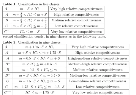
After computing the composite competitiveness indices Mereut¸˘a et all., 2007 consider two classifications. First classification consist in five classes as in the following table.

Table 1. Classification in five classes.

A+ _{m+S < IC}

i Very high relative competitiveness

A m+S

3 < ICi ≤m+S High relative competitiveness

B m₋S

3 < ICi ≤m+

S

3 Medium relative competitiveness

C m₋S < ICi ≤m− S₃ Low relative competitiveness

C−

ICi ≤m−S Very low relative competitiveness

Second classification consist in nine classes as in the following table.

Table 2. Classification in nine classes.

A++ _{m+ 1.75}

·S < ICi Very high relative competitiveness

A+ _{m+S < IC}

i ≤m+ 1.75·S High relative competitiveness

A m+ 0.5_·S < ICi ≤m+S Heigh-medium relative competitiveness

B+ _{m < IC}

i ≤m+ 0.5·S Medium-heigh relative competitiveness

B m₋0.5_·S < ICi ≤m Medium relative competitiveness

B−

m₋S < ICi ≤m−0.5·S Medium-low relative competitiveness

C m₋1.5_·S < ICi ≤m−S Low-medium relative competitiveness

C−

m₋1.75_·S < ICi ≤m−1.5·S Low relative competitiveness

C−−

ICi ≤m−1.75·S Very low relative competitiveness

In the above tables ICi is the composite competitive indice for the country i, m is the

average of the considered composite indice and S2 _{is its variance (hence S is its standard}

deviation). This is the reason of using of the formulae (13) and (14) in this paper: the eigenvalues λi are the variances of the new coordinates.

For the above classifications Mereut¸˘a et all., 2007 use the core method for obtaining the above tables. In this paper we will consider each classification in k classes (k = 5 or

k = 9 as in the above tables) using the backtracking method. From all these classifications (C8

26 = 1562275 for 9 classes and 27 countries) we choose that classification that optimizes

the considered criterion.

have countries with composite indices in inreasing order we compute first the separators of two successive classes as follows. Denote by Gi,i+1 the gravity center for the composite indices of

the classesiandi+ 1, and by mini, maxi, mini+1 and maxi+1 the minimum and the maximum

values of the considered composite indices for the class i, respectively for the class i+ 1. The separator of the classes i and i+ 1 is

sepi,i+1 =

        

       

Gi,i+1 if maxi ≤Gi,i+1 ≤mini+1

maxi if Gi,i+1 <maxi

mini+1 if Gi,i+1 >mini+1

min1 if i = 0

maxk if i =k

. (15)

Next we compute the probabilities of being in the class i

pi =

sepi,i+1−sepi−₁,i

sepk,k+1−sep0,1

, (16)

and from here we compute the entropy of the classification using (4).

Another criterion to select the optimal classification is the maximum Chow breakpoint statistics. Denoting by S2 _{the variance of all the classes for the considered composite indices}

and by S2

i the variance of the classi we compute the Chow statistics

Ch=

(n₋1)_·S2

−

k

P

i=1

(ni−1)·Si2 k

P

i=1

(ni−1)·Si2

· n−k

k−1, (17)

which has a Snedecor—Fisher with k₋1 andn₋k degrees of freedom. In the above formula we consider n countries classified in k classes such that the class i contains ni countries.

3

Application

Consider the GDP per capita (IC1), investment share in GDP (IC2), unemployment rate

(IC3), Gini index of income inequality (IC4) and share of consumption of renewal energy

resources (IC5) for the 27 countries of European Union.

Table 3. The correlated data.

Country AT BE BG CY CZ DK EE FI FR DE

V1 123.1 114.6 40.1 94.6 80.4 118.3 67.2 115 107.3 115.8

V2 21.8 22.7 33.4 23.3 24 21 28.4 20.6 21.9 19.2

V3 4.2 7.2 5.4 4.1 4.7 4.1 8.4 6.8 8.4 7.2

V4 29.1 33 29.2 33.45 25.4 24.7 35.8 26.9 32.7 28.3

V5 23.8 3.1 4.7 2.4 4.7 17.3 10 22.6 7 8.3

Country GR HU IE IT LV LT LU MT NL PL

V1 95.3 62.9 139.5 100.5 55.7 61.3 252.8 76.4 134.6 57.5

V2 19.3 20.1 21.1 20.9 30.2 24.8 20.1 15.8 20.5 22

V3 7.9 8.4 8.7 7 11.3 9 5.5 6.1 2.8 7.1

V4 34.3 26.9 34.3 36 37.7 36 34.6 26.15 30.9 34.5

V5 5 5.3 2.9 6.9 29.7 8.9 2.5 7.8 3.6 5.1

Country PT RO SK SI ES SE UK

V1 75.3 43.56 71.9 89.8 103.9 121.4 117.5

V2 21.7 33.3 25.9 28 29.4 19.5 16.9

V3 8.2 5.9 9.3 4.2 14.7 7 6.5

V4 38.5 31 25.8 28.4 34.7 25 36

V5 17.6 11.9 5.5 10 7 30.9 2.1

In the above table the GDP per capita and the share of investment in GDP are considred for the year 2008, the unemployment rate is considered for December 2008, the Gini index of incomes inequality is considered for 2007/2008 and the share of consumption of renewable energy resources are given for the year 2007.

For GDP per capita in the case of Romania the value of 45.8 is forecast for the year 2008, as the value 42.1 for 2007. But in Eurostat the value for Euro Area in 2008 is 108.9 and we know from ”Banca Nat¸ional˘a a Romˆaniei. Raport Anual 2008” that the Romanian GDP per capita is 40% from Euro Area, hence the value is 43.56.

The values of GDP per capita are also forecasted for the year 2008 in the cases of Austria, Greece and United Kingdom, and estimated for Slovakia. The Gini indexes lack for Cyprus, Luxembourg and Malta, but their values were computed as the neighbours’ average (the data in the source table are in order). Malta is also a lack in the table source of the share of consumption of renewable energy resources, but the value is replaced by the EU-27 average (7.8).

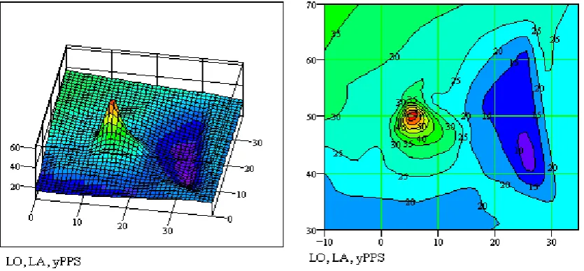
Euro PPS (Purchasing Power Standards). On the stylised map of the EU-27, we can see two distinct groups of regions delimited by 30 to 55 red contour lines and by 20 to 10 blue contour lines representing the highest and lowest GDP per capita levels respectively. In general, GDP per capita is increasing from the right side of EU-27 stylised map (eastern EU) to the left side (western EU) and from the bottom (southern EU) to the top (northern EU).

Source: own elaboration on EUROSTAT data.

Figure 1. 3-D map and contour plot of GDP per capital for EU-27 in 2006.

The variance-covariance matrix is         

1678.97444 ₋91.78076 21.77701 ₋3.94841 ₋35.05565 −91.78076 20.32617 ₋2.67091 ₋2.60698 3.38128

21.77701 −2.67091 5.95130 4.19329 −1.89291 −3.94841 −2.60698 4.19329 17.75154 5.70893 −35.05565 3.38128 ₋1.89291 5.70893 66.21525

        

with the eigenvalues

1685.09796, 66.14393, 20.5824, 13.24441 and 4.15001, and the eigenvectors on rows         

0.99816 ₋0.05509 0.01305 ₋0.00232 ₋0.02175 0.02328 0.02116 ₋0.01589 0.11273 0.993 0.03231 0.52199 ₋0.28595 ₋0.7995 0.0743 0.04475 0.84991 0.13084 0.50302 ₋0.07417 −0.00977 0.04122 0.94905 −0.30832 0.04954

         .

If we want to check the correlations between the five criteria we have to compute the

correlation matrix, which is         

1 ₋0.49682 0.21786 ₋0.02287 ₋0.07515 −0.49682 1 ₋0.24284 ₋0.13724 0.09217

0.21786 −0.24284 1 0.40797 −0.09536 −0.02287 ₋0.13724 0.40797 1 0.16652 −0.07515 0.09217 ₋0.09536 0.16652 1

        

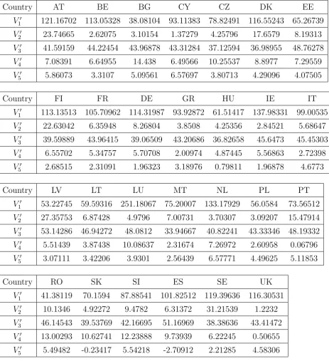
Table 4. The uncorrelated data.

Country AT BE BG CY CZ DK EE

V′

1 121.16702 113.05328 38.08104 93.11383 78.82491 116.55243 65.26739

V′

2 23.74665 2.62075 3.10154 1.37279 4.25796 17.6579 8.19313

V′

3 41.59159 44.22454 43.96878 43.31284 37.12594 36.98955 48.76278

V′

4 7.08391 6.64955 14.438 6.49566 10.25537 8.8977 7.29559

V′

5 5.86073 3.3107 5.09561 6.57697 3.80713 4.29096 4.07505

Country FI FR DE GR HU IE IT

V′

1 113.13513 105.70962 114.31987 93.92872 61.51417 137.98331 99.00535

V′

2 22.63042 6.35948 8.26804 3.8508 4.25356 2.84521 5.68647

V′

3 39.59889 43.96415 39.06509 43.20686 36.82658 45.6473 45.45303

V′

4 6.55702 5.34757 5.70708 2.00974 4.87445 5.56863 2.72398

V′

5 2.68515 2.31091 1.96323 3.18976 0.79811 1.96878 4.6773

Country LV LT LU MT NL PL PT

V′

1 53.22745 59.59316 251.18067 75.20007 133.17929 56.0584 73.56512

V′

2 27.35753 6.87428 4.9796 7.00731 3.70307 3.09207 15.47914

V′

3 53.14286 46.94272 48.0812 33.94667 40.82241 43.33346 48.19332

V′

4 5.51439 3.87438 10.08637 2.31674 7.26972 2.60958 0.06796

V′

5 3.07111 3.42206 3.9301 2.56439 6.57771 4.49625 5.11853

Country RO SK SI ES SE UK

V′

1 41.38119 70.1594 87.88541 101.82512 119.39636 116.30531

V′

2 10.1346 4.92272 9.4782 6.31372 31.21539 1.2232

V′

3 46.14543 39.53769 42.16695 51.16969 38.38636 43.41472

V′

4 13.00293 10.62741 12.23888 9.73939 6.22245 0.50655

V′

5 5.49482 -0.23417 5.54218 -2.70912 2.21285 4.58306

The performance indices are in the following table.

Table 5. The performance indices.

Country AT BE BG CY CZ DK EE

IC1 0.38989 0.35182 0 0.25825 0.1912 0.36824 0.12758

IC2 0.75098 0.0466 0.06263 0.00499 0.10119 0.54797 0.23239

IC3 0.39825 0.53541 0.52209 0.48792 0.16562 0.15852 0.77183

IC4 0.48823 0.45801 1 0.4473 0.70893 0.61445 0.50297

Country FI FR DE GR HU IE IT

IC1 0.3522 0.31736 0.35776 0.26207 0.10996 0.46881 0.2859

IC2 0.71376 0.17125 0.23489 0.08761 0.10104 0.05408 0.14881

IC3 0.29445 0.52185 0.26664 0.4824 0.15003 0.60953 0.59941

IC4 0.45157 0.3674 0.39242 0.13513 0.33448 0.38279 0.18483

IC5 0.58085 0.54055 0.50312 0.63519 0.37766 0.50371 0.79537

Country LV LT LU MT NL PL PT

IC1 0.07108 0.10095 1 0.17419 0.44626 0.08436 0.16651

IC2 0.87137 0.18842 0.12525 0.19285 0.08268 0.06231 0.47532

IC3 1 0.67701 0.73632 0 0.35818 0.48899 0.74216

IC4 0.37901 0.26489 0.69717 0.15649 0.50116 0.17687 0

IC5 0.62241 0.6602 0.71491 0.56785 1 0.77587 0.84288

Country RO SK SI ES SE UK

IC1 0.01549 0.15053 0.23371 0.29913 0.38158 0.36708

IC2 0.29712 0.12335 0.27524 0.16973 1 0

IC3 0.63548 0.29126 0.42822 0.89721 0.23128 0.49323

IC4 0.90013 0.73482 0.84697 0.67303 0.42829 0.03052

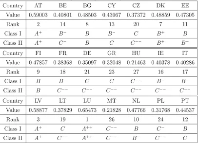
IC5 0.8834 0.2665 0.88849 0 0.52999 0.78522

For classification of the 27 countries we refer to ”Class I” if we use the maximum entropy criterion, and to ”Class II” for the Chow criterion. If we use the non-weighted indices we obtain the following table.

Table 6. Classification using non-weighted composite indices.

Country AT BE BG CY CZ DK EE

Value 0.59003 0.40801 0.48503 0.43967 0.37372 0.48859 0.47305

Rank 2 14 8 13 20 7 11

Class I A+ _B−

B B−

C B+ _B

Class II A+ _C−

B C C−−

B+ _B−

Country FI FR DE GR HU IE IT

Value 0.47857 0.38368 0.35097 0.32048 0.21463 0.40378 0.40286

Rank 9 18 21 23 27 16 17

Class I B B−

C C C−−

B−

B−

Class II B C−−

C−−

C−−

C−−

C−−

C−−

Country LV LT LU MT NL PL PT

Value 0.58877 0.37829 0.65473 0.21828 0.47766 0.31768 0.44537

Rank 3 19 1 26 10 24 12

Class I A+ _{C A}++ _C−−

B C−

B

Class II A+ _C−−

A++ _C−−

B−

C−−

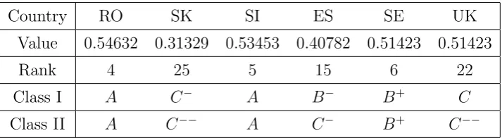
Country RO SK SI ES SE UK Value 0.54632 0.31329 0.53453 0.40782 0.51423 0.51423

Rank 4 25 5 15 6 22

Class I A C−

A B−

B+ _C

Class II A C−−

A C−

B+ _C−−

In the above table we have the same first four classes even we use the maximum entropy or the maximum separation: Luxembourg is alone in the first class, the second contains Austria and Latvia, the third contains Romania and Slovenia and the fourth contains Sweden and Denmark. The other countries from the rank 8 (Bulgaria) to the rank 27 (Hungary) are have the division in classes 5 + 6 + 5 + 2 + 2 in the case of maximum entropy, respectively 2+2+2+2+12 in the case of maximum separation. We notice in the last case the concentration of the last 12 countries in the last class.

The maximum entropy of the above classification (Class I) is 2.18454, very close to the maximum possible for 9 classes, namely ln 9 = 2.19722. The Chow statistics (Class II) is 1.89817 and it has a Snedecor—Fisher distribution with 8 and 18 degrees of freedom. If we compute the c.d.f. we obtain F (1.89817) = 0.87666 using the Simpson method (P˘altineanu et al., 1998), respectively F (1.89817) = 0.874 using the Monte Carlo method, simulating the normal random variables by the Box—Muler method (V˘aduva, 2004). Therefore in both cases the value of Chow statistics is grather than the centil of the order 0.13. For the above non-weighted indices we obtain the minimum 0.21463, the maximum 0.65473 and the variance 0.01158.

If we use the weighted indices we obtain the following table.

Table 7. Classification using weighted composite indices.

Country AT BE BG CY CZ DK EE

Value 0.33521 0.34072 0.13855 0.27813 0.22615 0.40514 0.23482

Rank 10 8 26 16 20 6 19

Class I B B C−−

B−

C−

B+ _C

Class II B−

B−

C−−

C−

C−

B+ _C−

Country FI FR DE GR HU IE IT

Value 0.41123 0.32369 0.34109 0.26003 0.13474 0.41869 0.30235

Rank 5 11 7 18 27 3 14

Class I B+ _{B B C C}−−

A B−

Class II B+ _{C B C}−

C−−

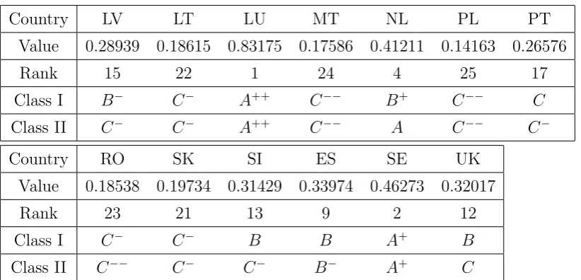
Country LV LT LU MT NL PL PT Value 0.28939 0.18615 0.83175 0.17586 0.41211 0.14163 0.26576

Rank 15 22 1 24 4 25 17

Class I B−

C−

A++ _C−−

B+ _C−−

C

Class II C−

C−

A++ _C−−

A C−−

C−

Country RO SK SI ES SE UK

Value 0.18538 0.19734 0.31429 0.33974 0.46273 0.32017

Rank 23 21 13 9 2 12

Class I C−

C−

B B A+ _B

Class II C−−

C−

C−

B−

A+ _C

In Figure 2 is presented the spatial distribution of Value (first row in the last table) in EU-27. In this case, we can see just a little different stylised map, signifying a more complex distribution within EU.

Source: own elaboration on EUROSTAT data.

Figure 2. 3-D map and contour plot of Value for EU-27.

When we use weighted composite indices instead of the non-weighted ones we can see that three countries remain on the same position: Luxembourg (first position), Czech Republic (position 20) and Hungary (last position, 27). We have also differences, the highest increasing being for Germany (14 positions from 21 to 7) and the highest decreasing being for Romania (19 positions from 4 to 23). The distribution of the 27 countries is 1+1+1+3+7+3+3+4+4 in the case of the maximum entropy, respectively 1 + 2 + 1 + 2 + 1 + 3 + 2 + 9 + 5 in the case of maximum separation. We notice that we have also higher concentration for the last classes in the case of maximum separation, as in the case of non-weighted composite indices.

4

Conclusions

We know (Onicescu and S¸tef˘anescu, 1979, Petric˘a and S¸tef˘anescu, 1982, Preda, 1992) that the maximum Shannon entropy for a simple random variable is reached for the uniform random variable. That’s why if we use the maximum entropy principle as classification criterion the countries are distributed into the classes as uniform as possible (there are not huge differences between the numbers of classes members).

In applications we use more the Chow statistics for which the first number of degree of freedom is greather than 1 (as in formula (12), for instance). This is the case of Chow breakpoint test, where the denominator is the estimated variance of the groups tacking into account the break points, and the numberator is the difference between the sum of squares if we do not consider the breakpoints and the same sum if we do, divided by the number of degrees of freedom. This is the logical explanation of the formula (17).

The selected performance criteria are in agreement with sustainable development (Indi-cators of Sustainable Development) and were approved by the Commission on Sustainable Development at its Third Session in 1995. We notice that each obtained eigenvector has at least one negative component, even the principal component. Therefore it is wrong to try to reduce all the costs or increase all the benefits if the values are correlated: for instance we can increase the value of the principal component by decreasing the investment share in GDP or by increasing the Gini index.

The new coordinates have positive values, except the last one (corresponding to the eigen-value 4.15001). In this case we have the values ₋0.23417 for Slovakia and ₋2.70912 for Spain.

If we want to apply the Chow breakpoint test in the considered application for non-weighted performance indices we accept the null hypothesis that we have no breakpoints even if the error level is 10% (0.87666<0.9), but the test is not the goal of using the Chow statistics: we want only to obtain the maximum of this statistics (the maximum separation). The weighted composite indices are more scattered than the non-weighted ones: in our example the minimum is less, and the maximum and the variance are greater in the first case. If we denote by σ2

1 the variance in the case of non-weighted composite indices, and by

σ2

2 the variance in the case of weighted composite indices we obtain

σ2 2

σ2 1 =

0.01958

0.01158 = 1.69117.

It is possible that this can explain also the lower Shannon entropy (hence the less uniform distribution) of the countries in the case of weighted indices.

References

[2] Chow, G.C. (Jul. 1960), ”Test Between Sets of Coefficients in Two Linear Regressions”,

Econometrica, Vol. 28, No. 3, pp. 591-605.

[3] Ciuiu, D., (2007), ”Pattern Classification using Principal Components Regression”, Pro-ceedings of the International Conference Trends and Challenges in Applied Mathematics, 20–23 June 2007, Technical University of Civil Engineering, Bucharest, Romania, pp. 149-152.

[4] Ciuiu, D., (2008), ”Pattern Classification using Secondary Components Perceptron and Economic Applications”,Romanian Journal of Economic Forecasting, No. 2, pp. 51-66.

[5] Jula, D., (2003), Introducere ˆın Econometrie, Ed. Professional Consulting, Bucure¸sti.

[6] Mereut¸˘a, C, Albu, L.L., Iordan, M. and Chilian, M.N., (2007), ”A Model to Evalu-ate the Regional Competitiveness of the EU Regions”, Romanian Journal of Economic Forecasting, No. 3, pp. 81-102.

[7] Onicescu, O. and S¸tef˘anescu, V. (1979),Elemente de statistic˘a informat¸ional˘a ¸si aplicat¸ii, Ed. Tehnic˘a, Bucure¸sti.

[8] P˘altineanu, G., Matei, P. and Trandafir, R., (1998), Analiz˘a numeric˘a, Ed. Conspress, Bucure¸sti.

[9] Petric˘a, I. and S¸tef˘anescu, V. (1982) Aspecte noi ale teoriei informat¸iei, Ed. Academiei, Bucure¸sti.

[10] Preda, V. (1992) Teoria deciziilor statistice, Ed. Academiei, Bucure¸sti.

[11] Saporta, G., (1990), Probabilit´es, Analyse des Don´ees et Statistique, Ed. Technip, Paris.

[12] V˘aduva, I. (2004), Modele de simulare, Ed. Universit˘at¸ii Bucure¸sti.

[13] Voineagu, V. et all, (2007), Teorie ¸si practic˘a econometric˘a, Meteor Press, Bucure¸sti.

[14] ”Banca Nat¸ional˘a a Romˆaniei. Raport Anual 2008”, www.bnr.ro/Publicatii-periodice-204.aspx.

[15] ”European Comission. Eurostat. Your Key to European Statistics”

[16] ”Indicators of Sustainable Development”, www.un.org/esa/sustdev/publications/indisd-mg2001.pdf.