Munich Personal RePEc Archive
On the Case for a Balanced Budget
Amendment to the U.S. Constitution
Marina, Azzimonti and Marco, Battaglini and Stephen,
Coate
U of Texas - Austin
2010
Online at
https://mpra.ub.uni-muenchen.de/25935/
Revised March 2010
Analyzing the Case for a Balanced Budget Amendment to the U.S.
Constitution
∗Abstract
This paper uses the political economy model of Battaglini and Coate (2008) to analyze the impact of a balanced budget rule that requires that legislators do not run deficits. It considers both a strict rule which cannot be circumvented and a rule that can be overridden by a super-majority of legislators. A strict rule leads to a gradual but substantial reduction in the level of public debt. In the short run, citizens will be worse off as public spending is reduced and taxes are raised to bring down debt. In the long run, the benefits of a lower debt burden must be weighed against the costs of greater volatility in taxes and less responsive public good provision. To quantify these effects, the model is calibrated to the U.S. economy using data from 1940-2005. While the long run net benefits are positive, they are outweighed by the short run costs of debt reduction. A rule with a super-majority override has no effect on citizen welfare orfiscal policy.
Marina Azzimonti Department of Economics University of Texas Austin TX 08544
Marco Battaglini
Department of Economics Princeton University Princeton NJ 08544 [email protected]
Stephen Coate
Department of Economics Cornell University Ithaca NY 14853 [email protected]
∗For research assistance we thank Kazuki Konno, Tim Lin, and Matthew Talbert. For helpful comments and
1
Introduction
A recurring debate in American politics concerns the desirability of amending the U.S. constitution
to require that the federal government operate under a balanced budget rule (BBR). Calls for such
a “balanced budget amendment” started in the late 1970s and became particularly strident during
the high deficit era in the 1980s and 1990s. Indeed, in 1995 the House approved a balanced budget
amendment by 300-132, but the Senate fell one vote short of the two-thirds majority that is needed
for constitutional amendments (Schick (2007)).1 Efforts to pass a balanced budget amendment
continued right up until the recent economic crisis and will doubtless resurface once the economy
recovers.2
While there is no shortage of policy discussion on the pros and cons of passing a balanced budget
amendment, there has been remarkably little economic analysis of its likely impact. Indeed, we
are not aware of anyanalysis that has tried to shed light, qualitatively or quantitatively, on the
likely impact onfiscal policy and citizen welfare. Doubtless this reflects the inherent difficulty of
developing an analysis that even begins to capture the key trade-offs. Since it is clear that in a
world in which policy is set by a benevolent planner a BBR can only distort policy and hurt citizen
welfare, one must begin with a political economy model offiscal policy. Moreover, the model must
be sufficiently rich to be able to capture the short and long run consequences of imposing a BBR
on policy and welfare.
The political economy model offiscal policy recently developed by Battaglini and Coate (2008)
(BC) appears a potentially useful framework in which to analyze the issue. The BC framework
begins with a tax smoothing model of fiscal policy of the form studied by Barro (1979), Lucas
and Stokey (1983), and Aiyagari et. al. (2002). It departs from the tax smoothing literature by
assuming that policy choices are made by a legislature rather than a benevolent planner. Moreover,
it incorporates the friction that legislators can redistribute tax dollars back to their districts via
1
The U.S. Constitution can be amended in two ways. Thefirst is by a two-thirds vote in both the House and Senate followed by ratification by three-fourths of the states. The second is by two-thirds of the states calling a Constitutional Convention at which three-fourths of the states must ratify the amendment. The latter route to adopting a balanced budget amendment was pursued in the late 1970s but fell four states short of the two-thirds necessary to call a Convention. See Morgan (1998) for a discussion of this effort.
2
pork-barrel spending. This friction means that equilibrium debt levels are too high implying that,
in principle, imposing a BBR has the potential to improve welfare.
In this paper, we employ the BC model to analyze the impact of imposing a BBR on the U.S.
federal government. Our hope is not only to contribute to the substantive debate concerning the
balanced budget amendment, but also to develop an appreciation for how useful the BC model
is for analyzing U.S. fiscal issues. The paper begins by calibrating the BC model to the U.S.
economy using data from 1940-2005 and argues that the calibrated modelfits the data sufficiently
well to make using it as a framework to underpin the policy analysis interesting.3 We then study,
both qualitatively and quantitatively, the consequences of imposing a BBR. We model a BBR as
a constitutional requirement that tax revenues must be sufficient to cover spending and the costs
of servicing the debt. Thus, budget surpluses are permitted, but not deficits.4 We consider both
a strict BBR which cannot be circumvented by the legislators and a BBR which can be overridden
by a super-majority of legislators.5
Imposing a strict BBR leads to a gradual reduction in the level of government debt. In the
calibrated model, the long run reduction in the debt/GDP ratio is 89%. This is surprising because
the BBR only restricts legislators not to run deficits and thus one might have expected the debt
level to remain constant. The reduction occurs because a BBR, by restricting future policies,
increases the expected cost of taxation and makes public savings more valuable as a buffer against
future shocks. The reduction in debt means that the interest costs of servicing debt will be lower,
reducing pressure on the budget. In the calibrated model, average tax rates become lower and
public good provision becomes higher than in the steady state of the unconstrained equilibrium.
Pork-barrel spending also becomes higher as debt falls. However, the inability to use debt to
smooth taxes, leads to more volatile tax rates and less responsive public good provision.
The impact of imposing a strict BBR on citizen welfare is complex. Initially, citizens experience
a reduction in average contemporaneous utility, as legislators reduce public spending and increase
3
This is thefirst calibration of the BC model to a real economy.
4
This is consistent with the balanced budget amendments that have been considered by Congress. As reported in Whalen (1995), the balanced budget amendment considered as part of the Contract with America in 1994 required that “total outlays for anyfiscal year do not exceed total receipts for that year”. Total receipts are defined as “all receipts of the United States except those derived from borrowing” and total outlays are defined as “all outlays of the United States except those for the repayment of debt principle”.
5
taxes to pay down debt. As debt declines, in principle they may or may not be better off. This
depends on whether the benefits of a lower debt burden are offset by the costs of more volatile
tax rates and less responsive public good provision. In the calibrated model, steady state welfare
is actually increased by 2.85%. However, when account is taken of the short run costs, imposing
a strict BBR reduces welfare.
The analysis of a BBR which can be overridden is much more straightforward: imposing a
BBR with a super-majority override will have no effect onfiscal policy or citizen welfare. Such
a BBR will only have an effect if imposed at the foundation of the state before debt has risen to
equilibrium levels. Intuitively, this is because in the BC model, once debt has reached equilibrium
levels, additional debt will be issued only when it is in the interests of all legislators to do so,
rather than just a minimum winning coalition. We argue that this result reflects the stationarity
of the BC model and would not necessarily apply in a growing economy.
The organization of the remainder of the paper is as follows. Section 2 provides a quick review
of the debate concerning the desirability of a balanced budget amendment and the academic
literature on BBRs. Section 3 briefly outlines the BC model offiscal policy. Section 4 explains
how we calibrate the model to the U.S. economy and discusses its suitability as a framework to
underpin the policy analysis. Section 5 studies, qualitatively and quantitatively, the impact of
imposing a strict BBR on equilibriumfiscal policies and welfare. Section 6 deals with the case of
a BBR with super-majority override. Section 7 discusses the results and Section 8 concludes.
2
Literature review
Advocates of a balanced budget amendment to the U.S. constitution see a BBR as a necessary tool
to limit the size of government and the level of public debt.6 Opponents argue that a BBR would
restrict government’s ability to use debt for beneficial purposes like tax smoothing, counter-cyclical
Keynesianfiscal policy, or public investment. Even if legislators tend to accumulate inefficiently
high debt levels, this does not mean that they will not use debt on the margin in ways that
enhance social welfare. Advocates respond that someflexibility may be preserved by allowing the
BBR to be overridden in times of war or with a supermajority vote of the legislature. Moreover,
6
investment expenditures might be exempted by the creation of separate capital budgets.7
A further common argument against a balanced budget amendment is that the BBR will be
circumvented by bookkeeping gimmicks and hence will be ineffective. Such gimmicks include the
establishment of entities, such as public authorities or corporations, that are authorized to borrow
money but whose debt is not an obligation of the state. Another gimmick involves selling public
assets and recording the proceeds as current revenue. Moreover, critics argue that this process of
circumvention will create a lack of transparency and accountability. Relatedly, critics fear that a
BBR might lead Congress to further their social objectives by inefficient non-budgetary measures.
For example, by imposing mandates on state and local governments or by imposing additional
regulations on the private sector. Finally, critics worry whether the enforcement of a BBR will
blur the line between the legislative and judicial branches of government.8
The academic literature that relates to the desirability of a balanced budget amendment has
largely been devoted to the empirical question of whether the BBRs that are used in practice
actually have any effect. Thus, the literature has honed in on the issue of the circumvention of
BBRs via accounting gimmicks and the like. Empirical investigation is facilitated by the fact that
BBRs are common at the state level in the U.S.. Moreover, not only is there significant variation
in the stringency of the different rules, but this variation is plausibly exogenous since many of the
states adopted their BBRs as part of their founding constitutions.9 Researchers have explored
how this stringency impactsfiscal policy (see, for example, Alt and Lowry (1994), Bayoumi and
Eichengreen (1995), Bohn and Inman (1996), Poterba (1994) and Rose (2006)). Importantly,
these studiesfind that stringency does matter forfiscal policy. For example, Poterba (1994) shows
that states with more stringent restraints were quicker to reduce spending and/or raise taxes in
response to negative revenue shocks than those without.10
Less work has been devoted to the basic theoretical question of whether, assuming that they
can be enforced and will not be circumvented, BBRs are desirable. In the optimalfiscal policy
literature, a number of authors point out that optimal policy will typically violate a BBR (see,
7
On separating capital and operating budgets see Bassetto with Sargent (2006).
8
On enforcement issues see Primo (2007).
9
Forty nine of the fifty U.S. states have some type of BBR (Vermont is the exception). Rhode Island was thefirst state to adopt a BBR in 1842 and thirty six more states adopted them before the end of the nineteenth century. See Savage (1988) for more on the history of BBRs and the importance of the balanced budget philosophy in American politics more generally.
10
for example, Lucas and Stokey (1983) and Chari, Christiano and Kehoe (1994)). In the context
of the model developed by Chari, Christiano and Kehoe (1994), Stockman (2001) studies how
a benevolent government would set fiscal policy under a BBR and quantifies the welfare cost of
such a restraint. However, by omitting political economy considerations, none of this work allows
for the possibility that a BBR might have benefits. Brennan and Buchanan (1980), Buchanan
(1995), Buchanan and Wagner (1977), Keech (1985) and Niskanen (1992) provide some interesting
discussion of the political economy reasons for a BBR, but do not provide frameworks in which to
evaluate the costs and benefits. Besley and Smart (2007) provide an interesting welfare analysis
of BBRs and other fiscal restraints within the context of a two period political agency model.
The key issue in their analysis is how having a BBR influences theflow of information to citizens
concerning the characteristics of their policy-makers. This is a novel angle on the problem to be
sure, but this argument has not, to this point, played a role in the policy debate.
In a precursor to this analysis, Battaglini and Coate (2008) briefly consider the desirability
of imposing a constitutional constraint at the foundation of the state that prevents government
from either running deficits or surpluses. They present a condition under which citizens will
be better offwith such a constraint. This condition concerns the size of the economy’s tax base
relative to the size of the public spending needs. The analysis in this paper goes beyond this initial
exploration in four important ways. First, it considers a BBR that allows for budget surpluses and
hence public saving or debt reduction. Second, it assumes that the BBR is imposed after debt has
reached equilibrium levels rather than at the beginning of time. Third, it calibrates the model to
the U.S. economy and develops quantitative predictions concerning the impact of a BBR. Fourth,
it considers a BBR with a super-majority override.
3
The BC model
3.1
The economic environment
A continuum of infinitely-lived citizens live inn identical districts indexed byi = 1, ..., n. The
size of the population in each district is normalized to be one. There is a single (nonstorable)
consumption good, denoted byz, that is produced using a single factor, labor, denoted byl, with
the linear technologyz =wl. There is also a public good, denoted by g, that can be produced
Citizens consume the consumption good, benefit from the public good, and supply labor. Each
citizen’s per period utility function is
z+Alng−l(1+1ε+ 1/ε), (1)
where ε > 0. The parameterA measures the value of the public good to the citizens. Citizens
discount future per period utilities at rateδ.
The value of the public good varies across periods in a random way, reflecting shocks to the
society such as wars and natural disasters. Specifically, in each period, Ais the realization of a
random variable with range [A, A] and cumulative distribution functionG(A). The functionGis
continuously differentiable and its associated density is bounded uniformly below by some positive
constantξ >0, so that for any pair of realizations such thatA < A0, the differenceG(A0)−G(A) is
at least as big asξ(A0−A).
There is a competitive labor market and competitive production of the public good. Thus, the
wage rate is equal towand the price of the public good is p. There is also a market in risk-free,
one period bonds. The assumption of a constant marginal utility of consumption implies that the
equilibrium interest rate on these bonds must beρ= 1/δ−1.
3.2
Government policies
The public good is provided by the government. The government can raise revenue by levying
a proportional tax on labor income. It can also borrow and lend by selling and buying bonds.
Revenues can also be diverted tofinance targeted district-specific monetary transfers which are
interpreted as (non-distortionary) pork-barrel spending.
Government policy in any period is described by ann+ 3-tuple{τ, g, b0, s
1, ...., sn}, whereτis
the income tax rate;gis the amount of public good provided;b0 is the amount of bonds sold; and
siis the transfer to districti’s residents. Whenb0 is negative, the government is buying bonds. In
each period, the government must also repay the bonds that it sold in the previous period which
are denoted byb. The government’s initial debt level in period 1 isb0.
In a period in which government policy is{τ, g, b0, s
1, ...., sn}, each citizen will supplyl∗(τ) =
(εw(1−τ))ε units of labor. A citizen in district i who simply consumes his net of tax earnings
and his transfer will obtain a per period utility ofu(τ, g;A) +si, where
u(τ, g;A) = ε
ε(w(1−τ))ε+1
Since citizens are indifferent as to their allocation of consumption across time, their lifetime
expected utility will equal the value of their initial bond holdings plus the payoff they would
obtain if they simply consumed their net earnings and transfers in each period.
Government policies must satisfy three feasibility constraints.11 First, tax revenues must be
sufficient to cover public expenditures. To see what this implies, consider a period in which the
initial level of government debt isb and the policy choice is {τ, g, b0, s
1, ...., sn}. Expenditure on
public goods and debt repayment ispg+ (1 +ρ)b, tax revenue isR(τ) =nτ wl∗(τ), and revenue
from bond sales isb0. Letting thenet of transfer surplusbe denoted by
B(τ, g, b0;b) =R(τ)−pg+b0−(1 +ρ)b, (3)
the constraint requires thatB(τ, g, b0;b)≥X
isi. Second, district-specific transfers must be
non-negative (i.e., si ≥ 0 for all i). Third, the government cannot borrow more than it can repay
which requires thatb0 is less thanb= max
τR(τ)/ρ.
3.3
The political process
Government policy decisions are made by a legislature consisting of representatives from each of
thendistricts. One citizen from each district is selected to be that district’s representative. Since
all citizens have the same policy preferences, the identity of the representative is immaterial and
hence the selection process can be ignored. The legislature meets at the beginning of each period.
These meetings take only an insignificant amount of time, and representatives undertake private
sector work in the rest of the period just like everybody else. The affirmative votes of q < n
representatives are required to enact any legislation.
To describe how legislative decision-making works, suppose the legislature is meeting at the
beginning of a period in which the current level of public debt isband the value of the public good
isA. One of the legislators is randomly selected to make thefirst proposal, with each representative
having an equal chance of being recognized. A proposal is a policy{τ, g, b0, s
1, ...., sn}that satisfies
the feasibility constraints. If thefirst proposal is accepted byqlegislators, then it is implemented
and the legislature adjourns until the beginning of the next period. At that time, the legislature
11
There is also an additional constraint that the total amount of private sector income be larger than the amount borrowed by the government. This requires thatPisi+ (1 +ρ)b+n(1−r)w(εw(1−r))ε exceedb0. Using the
budget balance condition for the government, this constraint amounts to the requirement that national income
nw(εw(1−r))ε exceed public good spendingpg. This condition is easily satisfied in the calibration of the model
meets again with the difference being that the initial level of public debt isb0 and there is a new
realization of A. If, on the other hand, the first proposal is not accepted, another legislator is
chosen to make a proposal. There areT ≥2 such proposal rounds, each of which takes a negligible
amount of time. If the process continues until proposal roundT, and the proposal made at that
stage is rejected, then a legislator is appointed to choose a default policy. The only restrictions
on the choice of a default policy are that it be feasible and that it treats districts uniformly (i.e.,
si=sj for alli,j).
3.4
Political equilibrium
Battaglini and Coate study the symmetric Markov-perfect equilibrium of this model. In this type
of equilibrium, any representative selected to propose at roundr ∈ {1, ..., T}of the meeting at
some time t makes the same proposal and this depends only on the current level of public debt
(b), the value of the public good (A), and the bargaining round (r). Legislators are assumed to
vote for a proposal if they prefer it (weakly) to continuing on to the next proposal round. It is
assumed, without loss of generality, that at each roundrproposals are immediately accepted by
at least qlegislators, so that on the equilibrium path, no meeting lasts more than one proposal
round. Accordingly, the policies that are actually implemented in equilibrium are those proposed
in thefirst round.
3.4.1 Characterization of equilibrium
To understand equilibrium behavior note that to get support for his proposal, the proposer must
obtain the votes ofq−1 other representatives. Accordingly, given that utility is transferable, he is
effectively making decisions to maximize the utility ofqlegislators. It is thereforeas ifa randomly
chosen minimum winning coalition (mwc) ofqrepresentatives is selected in each period and this
coalition chooses a policy choice to maximize its aggregate utility.
In any given state (b, A), there are two possibilities: either the mwc will provide pork to the
districts of its members or it will not. Providing pork requires reducing public good spending or
increasing taxation in the present or the future (if financed by issuing additional debt). When
b and/or A are sufficiently high, the marginal benefit of spending on the public good and the
marginal cost of increasing taxation may be too high to make this attractive. In this case, the
legislature as a whole.
If the mwc does provide pork, it will choose a tax rate-public good-public debt triple that
maximizes coalition aggregate utility under the assumption that they share the net of transfer
surplus. Thus, (τ, g, b0) solves the problem:
maxu(τ, g;A) +B(τ,g,bq 0;b)+δEv(b0, A0)
s.t. b0 ≤b,
(4)
where v is the continuation value function. The optimal policy is (τ∗, g∗(A), b∗) where the tax
rateτ∗ satisfies the condition that
1
q =
[ 1−τ∗
1−τ∗(1+ε)]
n , (5)
the public good levelg∗(A) satisfies the condition that
A g∗(A)=
p
q, (6)
and the public debt levelb∗ satisfies
b∗= arg max{b 0
q +δEv(b
0, A0) :b0
≤b}. (7)
To interpret condition (5) note that (1−τ)/(1−τ(1 +ε)) measures the marginal cost of taxation
-the social cost of raising an additional unit of revenue via a tax increase. It exceeds unity whenever
the tax rate (τ) is positive, because taxation is distortionary. Condition (5) therefore says that
the benefit of raising taxes in terms of increasing the per-coalition member transfer (1/q) must
equal the per-capita cost of the increase in the tax rate. Condition (6) says that the per-capita
benefit of increasing the public good must equal the per-coalition member reduction in transfers
it necessitates. Condition (7) says that the level of borrowing must optimally balance the benefits
of increasing the per-coalition member transfer with the expected future costs of higher debt next
period. We will discuss this condition further below.
The mwc will choose pork if the net of transfer surplus at this optimal policyB(τ∗, g∗(A), b∗;b)
is positive. Otherwise the coalition will provide no pork and its policy choice will maximize
aggregate legislator (and hence citizen) utility. Conveniently, the equilibrium policies turn out to
Proposition 1. The equilibrium value functionv(b, A)solves the functional equation
v(b, A) = max
(τ,g,b0)
⎧ ⎪ ⎪ ⎨ ⎪ ⎪ ⎩
u(τ, g;A) +B(τ,g,bn 0;b)+δEv(b0, A0) :
B(τ, g, b0;b)≥0,τ ≥τ∗,g≤g∗(A), &b0∈[b∗, b] ⎫ ⎪ ⎪ ⎬ ⎪ ⎪ ⎭
(8)
and the equilibrium policies{τ(b, A),g(b, A),b0(b, A)}are the optimal policy functions for this
pro-gram.
The objective function in problem (8) is average citizen utility. A social planner would therefore
maximize this objective function without the constraints on the tax rate, public good level and
debt. Thus, political determination simply amounts to imposing three additional constraints on
the planning problem. The only complication is that the lower bound on debt b∗ itself depends
upon the value function via equation (7) and hence is endogenous.
Given Proposition 1, it is straightforward to characterize the equilibrium policies. Define the
functionA∗(b, b0) from the equationB(τ∗, g∗(A), b0;b) = 0.Then, if the state (b, A) is such that
Ais less than A∗(b, b∗) the tax-public good-debt triple is (τ∗, g∗(A), b∗) and the mwc shares the
net of transfer surplusB(τ∗, g∗(A), b∗;b). IfAexceedsA∗(b, b∗) the budget constraint binds and
no transfers are given. The tax-debt pair exceeds (τ∗, b∗) and the level of public good is less than
g∗(A). The solution in this case can be characterized by obtaining the first order conditions for
problem (8) with only the budget constraint binding. The tax rate and debt level are increasing
inb andA, while the public good level is increasing inAand decreasing inb.
The characterization in Proposition 1 takes as fixed the lower bound on debt b∗ but as we
have stressed this is endogenous. Taking thefirst order condition for problem (7) and assuming
an interior solution, we see thatb∗ satisfies
1
q =−δE[
∂v(b∗, A0)
∂b0 ]. (9)
This tells us that the marginal benefit of extra borrowing in terms of increasing the per-coalition
member transfer must equal the per-capita expected marginal cost of debt. Using Proposition 1
and the Envelope Theorem, it can be shown that:
−δE[∂v(b
∗, A)
∂b0 ] = [G(A
∗(b∗, b∗)) +Z A
A∗(b∗,b∗)(
1−τ(b∗, A)
1−τ(b∗, A)(1 +ε))dG(A)]/n. (10)
The intuition is this: in the event that A is less than A∗(b∗, b∗) in the next period, increasing
a per-capita cost of 1/n. By contrast, in the event thatAexceedsA∗(b, b∗), there is no pork, so
reducing debt means increasing taxes. This has a per-capita cost of (1−τ)/[n(1−τ(1 +ε))] when
the tax rate isτ.
Substituting (10) into (9), observe that since 1/q >1/n, for (9) to be satisfied,A∗(b∗, b∗) must
lie strictly betweenAandA. Intuitively, this means that the debt levelb∗ must be such that next
period’s mwc will provide pork with a probability strictly between zero and one.
3.4.2 Equilibrium dynamics
The long run behavior offiscal policies in the political equilibrium is summarized in the following
proposition:
Proposition 2. The equilibrium debt distribution converges to a unique, non-degenerate invariant
distribution whose support is a subset of[b∗, b). When the debt level is b∗, the tax rate isτ∗, the
public good level isg∗(A), and a minimum winning coalition of districts receive pork. When the
debt level exceeds b∗, the tax rate exceeds τ∗, the public good level is less than g∗(A), and no
districts receive pork.
In the long run, equilibriumfiscal policiesfluctuate in response to shocks in the value of the public
good. Legislative policy-making oscillates between periods of pork-barrel spending and periods of
fiscal responsibility. Periods of pork are brought to an end by high realizations in the value of the
public good. These trigger an increase in debt and taxes tofinance higher public good spending
and a cessation of pork. Once in the regime of fiscal responsibility, further high realizations of
Atrigger further increases in debt and higher taxes. Pork returns only after a suitable sequence
of low realizations of A. The larger the amount of debt that has been built up, the greater the
expected time before pork re-emerges.
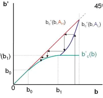
Figure 1 illustrates the dynamic evolution of debt under the assumption that there are just
two public good shocks, high and low, denoted AH and AL. The horizontal axis measures the
initial debt levelb and the vertical the new levelb0. The dashed line is the 45o line. The Figure
depicts the two policy functionsb0(b, A
H) andb0(b, AL). In thefirst period, given the initial debt
level b0, debt jumps up to b∗ irrespective of the value of the shock. In the second period, debt
remains atb∗ if the shock is low, but increases if the shock is high. It continues to increase for
as long as the shock is high. When the shock becomes low, debt starts to decrease, eventually
Figure 1: Evolution of debt
The debt levelb∗ plays a key role in equilibrating the system. If it is positive, the economy is
in perpetual debt, with the extent of debt spiking up after a sequence of high values of the public
good. When it is negative, the government will have positive asset holdings at least some of the
time. The key determinant ofb∗ is the size of the tax base as measured byR(τ∗) relative to the
economy’s desired public good spending as measured bypg∗(A). The greater the relative size of
the tax base, the larger isb∗.12
It is instructive to compare the equilibrium behavior with the planning solution for this
econ-omy. The latter is obtained by solving problem (8) without the lower bound constraints on taxes
and debt, and the upper bound constraint on public goods. The solution involves the government
gradually accumulating sufficient bonds so as to always be able tofinance the Samuelson level of
the public good solely from the interest earnings. Thus, in the long run, the tax rate is equal to
zero. In each period, excess interest earnings are rebated back to citizens via a uniform transfer.
4
Calibration to the U.S.
This section describes how to compute the political equilibrium of the BC model and how we
calibrate it to the U.S. economy. It then discusses thefit of the model and performs some
simu-12
lations to see how well the model captures the behavior of the keyfiscal policy variables. Some
limitations of the model are also discussed.
4.1
Numerical implementation and computation
The “state-space” of the BC model is the set of (b, A) pairs such that b ≤ b and A ∈ [A, A].
We discretize this state-space by assuming that the preference shock A belongs to a finite set
A={A1, ..., AI}and requiring that the debt levelbbelongs to thefinite setB={b1, ..., bu}. We
assume that the lowest debt levelb1 is equal to the level that a planner would choose in the long
run; that is,b1=−pgS(AI)/ρwheregS(AI) is the Samuelson level of the public good associated
with the maximal shockAI. We will discuss how the maximum debt levelbu is chosen below.
The characterization in Proposition 1 suggests a simple algorithm to compute the
laissez-faire equilibrium. Given a value of b∗, (8) is a functional equation that can be solved for the
equilibrium value functionv(b, A). The equation has a unique solution since the mapping defined
by the maximization on the right hand side of (8) is a contraction. The only difficulty is that the
lower boundb∗is endogenously determined along with the value function. However, this difficulty
can be overcome by exploiting the fact thatb∗ solves the maximization problem described in (7).
These observations motivate the following computational procedure:
• Step 1. Choose some z ∈ B as a value for b∗ and obtain the values τ∗ and g∗(A) from
equations (5) and (6) respectively.
• Step 2. Solve forvz by iterating on the value function below
vz(b, A) = max
(τ,g,b0)
⎧ ⎪ ⎪ ⎨ ⎪ ⎪ ⎩
u(τ, g) +Alng+B(τ,g,bn 0;b)+δEvz(b0, A0)
B(τ, g, b0;b)≥0,g≤g∗(A),τ≥τ∗, & b0 ∈[z, b
u].
⎫ ⎪ ⎪ ⎬ ⎪ ⎪ ⎭
• Step 3. Calculate
arg max{b0/q+δEvz(b0, A0) :b0∈B}.
• Step 4. If the optimal value calculated in Step 3 is notz, select anotherz ∈Bas a value
forb∗and repeat the procedure. If the optimal value isz, thenzis the estimate ofb∗andvz
is the estimated equilibrium value function.13 The equilibrium policy functions can then
13
be obtained by solving the constrained planning problem described in Step 2.
Effectively, our computational procedure searches for ab∗that is afixed point of the above system.
Intuitively, we are searching for the value of b∗ that determines a value function for which the
mwc would actually choose to borrowb∗ when providing pork to its members.
In our numerical implementation, we use a 200-point grid A for the preference shocks. We
choose the gridB for debt so that further increases in the number of points neither change the
lower bound b∗ nor the value of the key statistics we attempted to match (more detail on this
when discussing the calibration). The resulting set B has 4000 non-evenly spaced grid points,
which are more concentrated at values of debt greater than zero. A global approximation method
is used in the computation of the equilibrium.
4.2
Calibration
We normalize the number of districts to n= 100. Consistent with Cooley and Prescott (1995),
we set the discount factorδ equal to 0.95. This implies that the annual interest rate on bondsρ
is 5.26%. Following Aiyagari et. al. (2002) and consistent with the measure used in Greenwood,
Hercowitz and Huffman (1988) for a similar disutility of labor function, we assume the elasticity
of labor supplyεis equal to 2. The wage ratewis normalized so that the value of GDP when the
tax rate isτ∗ is 100. This implies a value of wequal to 0.72. Finally, the relative price of public
to private goodspis set equal to 1.
In terms of the shock structure, we assume that in any period, the economy can be in one of
two regimes: “normal times” or “extraordinary times”. The former captures shocks to spending
that occured mostly in the post-war period (including medium size wars such as Vietnam and
Iraq), while the latter tries to capture the extraordinary expenditure levels that occured during
World War II. In normal times,Ais log-normally distributed with meanμand varianceθ2, so that
log(A)∼N(μ, θ2). In extraordinary times, log(A) is equal to μ
w> μimplying that the demand
for public good provision (i.e., defense) is higher. The assumption that there is no volatility in
Aduring extraordinary times is just made for simplicity. We further assume that the economy is
in normal times 95.5% of the time and in extraordinary times 4.5% of the time. This is because
there were three years during our 66 year sample (the World War II years 1942-45) in which
government spending was particularly large. In normal times, the shocks are discretized using
We calibrate five parameters in all: the three parameters of the shock distribution μ, μw,
and θ; the required number of votes needed for a proposal to be approved by the legislature q;
and the upper bound on debtbu. While it may seem natural to setq equal to 51%, in the U.S.
context super-majority approval of budgets will typically be necessary to overcome the threats
of presidential vetos or Senate filibusters. Rather than trying to guess an appropriate value
based on institutional considerations, we decided to inferqfrom the data. We choose to calibrate
bu because setting it equal to the theoretical upper bound on debt b = maxτR(τ)/ρ creates
difficulties matching all the moments. In particular, the average debt/GDP ratio predicted by
the model is too high. We think that this reflects the fact that the theoretical upper bound is
unrealistically high. More specifically, since repayingbwould imply setting all future public good
provision equal to zero, we suspect that the government would in fact default if saddled with this
amount of debt. We are not sure what is the true maximum amount the government could borrow
and so, again, we try to infer it from the data.
We choose ourfive parameters to matchfive target moments in the data. Thefirst two targets
are the normal times (i.e., excluding the World War II years) mean and variance of government
spending as a proportion of GDP in the U.S. during the period 1940-2005. The third is the
maximum value of government spending as a proportion of GDP. Thefinal two are the average
and maximum ratio of government debt to GDP during 1940-2005.14 Ourfive parameters are
chosen so that the model generates, under the stationary distribution, close to the same values
that are observed in the data. The resulting values, together with other relevant parameters, are
listed in Table 1.
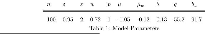
n δ ε w p μ μw θ q bu
[image:17.612.96.444.529.587.2]100 0.95 2 0.72 1 -1.05 -0.12 0.13 55.2 91.7 Table 1: Model Parameters
14
4.3
Model
fi
t
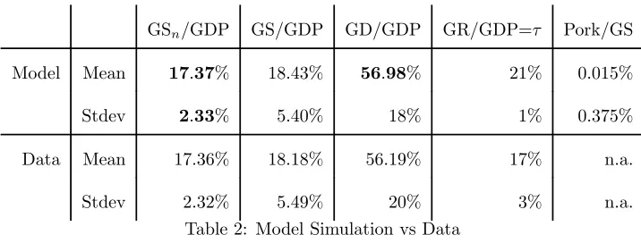
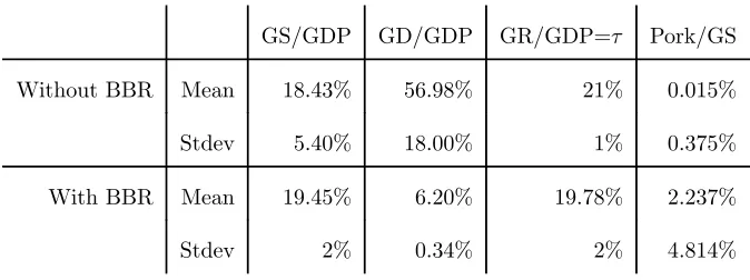
Table 2 summarizes the model’sfit for a set of selected variables that compose the government’s
budget. The first column reports government spending as a percentage of GDP during normal
times (GSn/GDP), while the second column includes the war years (GS/GDP). The third column
reports the ratio of government debt to GDP (GD/GDP), while the fourth reports government
revenue as a proportion of GDP (GR/GDP). In our model, the latter is simply the proportional
income tax rateτ.
The top two rows report the model’s simulated means and variances, and the bottom two rows
their counterparts in the data. The model’s statistics are based on a numerical approximation to
the theoretical invariant distribution of debt.15 The mean and standard deviation of normal times
spending as a ratio of GDP (listed in bold in the first column), as well as the mean debt/GDP
ratio (listed in bold in the third column), are three of ourfive target values, and thus match the
data well by construction.
GSn/GDP GS/GDP GD/GDP GR/GDP=τ Pork/GS
Model Mean 17.37% 18.43% 56.98% 21% 0.015%
Stdev 2.33% 5.40% 18% 1% 0.375%
Data Mean 17.36% 18.18% 56.19% 17% n.a.
[image:18.612.127.485.372.508.2]Stdev 2.32% 5.49% 20% 3% n.a.
Table 2: Model Simulation vs Data
The mean government spending/GDP ratio during World War II was also one of our target
moments. The model delivers 40.5% while the data counterpart is 40%. Note that the mean of
government spending/GDP (second column) predicted by the model matches the data well. Since
this mean is a combination of the two conditional means (normal times and extraordinary times),
with the weights determined by the probability of war, this suggests that our approximation of
the shock process is accurate.
Consistent with tax smoothing principles, we see from Table 2 that the volatility of the
gov-ernment debt/GDP ratio in the data is much higher than that of the govgov-ernment revenue/GDP
15
ratio (20% for the former, 3% for the latter). Despite the fact that we did not directly target the
debt/GDP volatility, the model generated a value quantitatively similar to that observed in the
data. The predicted volatility of revenue/GDP is much lower than in the data suggesting that
there is more tax smoothing going on in the model than in the actual economy. Nonetheless, the
average revenue/GDP ratio generated by the model is very much in line with the data. The last
column shows the long-run average level of pork as a proportion of total spending. This low value
reflects the fact that in the long run debt is rarely at a level that makes pork likely.16 The
dis-crepancy associated with this prediction is difficult to assess without a clear way of distinguishing
pork and public goods empirically.
There are two other statistics not reported in Table 2 that are nonetheless important to
men-tion. Thefirst one, is the targeted maximum debt/GDP ratio. The model delivers an expected
value of the maximum debt/GDP ratio of 120.6%, very close to the 121% observed in the data.
The second statistic, not a target value, is the lower bound on the debt/GDP ratio. In the data,
during the period 1940-2005 this was never below 31.5%. Encouragingly, the lower bound
gen-erated by the model–calculated asb∗/E(y)–is 29.4%. Thus, the political frictions captured by
the model generate quantitatively a realistic and endogenous lower bound for debt. Moreover,
the long-run stationary distribution of debt/GDP that our model generates is in line with that
observed in the U.S. as seen in Figure 2.
The fact that the model delivers such a goodfit with the actual distribution of the debt/GDP
ratio should not be overlooked. It is very difficult to explain the observed debt distribution with
a normative model. As noted earlier, the planner’s solution converges to a steady state where
the government has sufficient assets to finance the Samuelson level of the public good with the
interest earnings and taxes are zero. Obviously such a prediction is untenable. Aiyagari et. al
(2002) showed that a non-degenerate distribution for debt could be generated by imposing an
ad-hoc lower bound on debt (i.e., an upper limit on how many assets the government could hold).
However, as they observe, it is not clear why the government should face such a constraint. The
BC model provides a theoretical resolution of this difficulty and our calibration shows that, for
the U.S., this resolution works rather nicely empirically.
16
The probability that pork is provided when the debt level isbisG(A∗(b, b∗)). Equations (9) and (10) tell us
that this probability must be reasonably large whenb=b∗but it turns out to decrease sharply for largerb. Thus,
0.3 0.4 0.5 0.6 0.7 0.8 0.9 1 1.1 0
0.02 0.04 0.06 0.08 0.1 0.12 0.14 0.16 0.18
b/y
p
Histogram US debt/GDP
[image:20.612.179.420.139.334.2]Model US Data
Figure 2: Stationary distribution of debt/GDP
4.4
Simulations
To test how well the model captures the behavior of the key policy variables, we simulated the
economy for the period 1940-2005. As an initial condition, we assumed that debt/GDP in the
model was identical to that in the data. We further assumed that the economy was in normal
times until 1942, where we hit the system with an extraordinary times shock for three years. After
that, we assume the economy remains in normal times for the remainder of the sample. Given the
initial value ofband the sequence of shocks, we computed the evolution of government spending,
revenues, and debt.
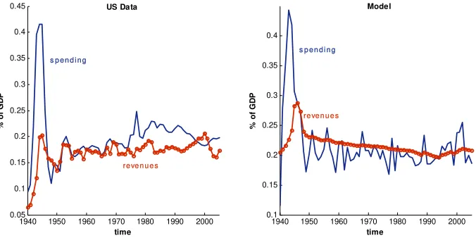
The left hand panel of Figure 3 shows the time paths of spending and revenue as a proportion
of GDP in the data. Revenues are much more stable than spending reflecting the government’s
tax smoothing. The right hand side show the impulse-responses from the model. The Figure
shows the model nicely replicates the tax smoothing behavior observed in the data.
The U.S. government financed the massive increase in public spending during World War II
largely by issuing debt. The increase in the government debt/GDP ratio can be seen in Figure 4,
which also depicts the behavior of debt for our simulated economy. Notice that the model captures
1940 1950 1960 1970 1980 1990 2000 0.05
0.1 0.15 0.2 0.25 0.3 0.35 0.4 0.45
time
% o
f
G
D
P
US Data
1940 1950 1960 1970 1980 1990 2000
0.1 0.15 0.2 0.25 0.3 0.35 0.4
time
% o
f
G
D
P
Model
re ve n u e s s p e n d i n g
[image:21.612.137.475.138.312.2]re ve n u e s s p e n d i n g
Figure 3: Response to a war shock, data (left panel) vs model (right panel)
decreased rapidly after the shock, the level of debt drops back at a much lower speed. While we
capture this qualitatively, our model over-predicts debt persistence. This may be due to the fact
that the model abstracts from changes in the growth rate experienced by the U.S. in the 1950s.
The model also has difficulty in explaining the up-turn in the debt/GDP ratio in the mid 1980s.17
4.5
Some limitations
We feel that the calibrated BC model provides a surprisingly good fit of the data given its
sim-plicity. In particular, thefit of the debt distribution illustrated in Figure 2 is very encouraging.
This provides some justification for using the model to analyze how imposing a balanced budget
amendment would impact the U.S. economy. Nonetheless, the model has many limitations and
we discuss four of the most important ones here.
Although dynamic, the BC model does not allow for persistent growth. Since there has been
substantial growth in the U.S. economy over the period in question, to calibrate the model it
is necessary to match the predictions of the model concerning policies as a proportion of GDP
17
1940 1950 1960 1970 1980 1990 2000 2010 0.4
0.5 0.6 0.7 0.8 0.9 1 1.1 1.2
year
% o
f
G
D
P
[image:22.612.201.413.140.318.2]US data Model
Figure 4: Response of debt to a war
with the data on policies as a proportion of GDP. Matching policylevels, even when corrected for
inflation, would not be possible. But this raises the question of whether the equilibrium behavior of
fiscal policies that the model predicts would emerge in a growing economy. For example, would the
debt/GDP ratio in a growing economy behave the same as the debt/GDP ratio in the stationary
economy? This is an open question.
A second limitation concerns entitlements spending. We included Social Security and Medicare
spending in our computation of the government spending/GDP ratio. Expenditure on these
programs has grown significantly since World War II and this is primarily responsible for the
upward trend in the spending/GDP ratio exhibited in the left panel of Figure 3. In calibrating
the model, we target the average spending/GDP ratio over the entire 1940-2005 period. Thus,
our shock structure does not incorporate the increase in spending observed in the latter part of
our sample period.
A third limitation concerns the assumed constant marginal utility of consumption. This
as-sumption means that, given the interest rateρ, citizens are indifferent over the time path of their
consumption. This results in consumption being more volatile in the model than in the data.18
The assumption also implies that the interest rate is constant so that the model cannot capture
18
variations in interest rates.19
A final limitation concerns the neglect of counter-cyclical fiscal policy. Since the recession
began in 2008, the debt/GDP ratio has risen sharply in the U.S.. In part, this has reflected
efforts to stimulate the economy via Keynesian pump-priming. This important motive for deficit
spending is absent from the model.20
5
The impact of a strict BBR
We are now ready to analyze the impact of imposing a strict BBR on the economy. We model a
strict BBR as a requirement that tax revenues must always be sufficient to cover spending and
the costs of servicing the debt. If the initial level of debt isb, this requires that
R(τ)≥pg+X
i
si+ρb. (11)
Given the definition ofB(τ, g, b0;b) (see (3)), a BBR is equivalent to adding, in each period, the
feasibility constraint thatb0≤b; i.e., that debt cannot increase. Thus, under a BBR, next period’s
feasible debt levels are determined by this period’s debt choice. In particular, if debt is paid down
in the current period, that will tighten the debt constraint in the next period. Wefirst study what
can be said qualitatively about the impact of a BBR and then turn to the calibrated model.
5.1
Qualitative analysis
Under a BBR, the equilibrium will still have a recursive structure. Let{τc(b, A),gc(b, A),b0c(b, A)}
denote the equilibrium policies under the constraint and vc(b, A) the value function. As in the
unconstrained equilibrium, in any given state (b, A), either the mwc will provide pork to the
districts of its members or it will not. If the mwc does provide pork, it will choose a tax-public
good-debt triple that maximizes coalition aggregate utility under the assumption that they share
19
In addition, with a diminishing marginal utility of consumption, the government will have incentives to manipulate the interest rate in its favor. Given a lack of commitment, this would cause further distortions in a political equilibrium. For a discussion of this, see Lucas and Stokey (1983) for the benevolent planner case, and Azzimonti, deFrancisco and Krusell (2007) for an analysis under majority voting.
20
the net of transfer surplus. Thus, (τ, g, b0) solves the problem:
maxu(τ) +Alng+B(τ,g,bq 0;b)+δEvc(b0, A0)
s.t. b0 ≤b.
The optimal policy is (τ∗, g∗(A), b∗
c(b)) where the tax rateτ∗ and public good levelg∗(A) are as
defined in (5) and (6), and the public debt levelb∗
c(b) satisfies
b∗c(b)∈arg max{b 0
q +δEvc(b
0, A0) :b0≤b}. (12)
As in the case without a BBR, if the mwc does not provide pork, the outcome will be as if it
is maximizing the utility of the legislature as a whole. Following the logic of Proposition 1, we
obtain:
Proposition 3. Under a strict BBR, the equilibrium value functionvc(b, A)solves the functional
equation
vc(b, A) = max
(τ,g,b0)
⎧ ⎪ ⎪ ⎨ ⎪ ⎪ ⎩
u(τ) +Alng+B(τ,g,bn 0;b)+δEvc(b0, A0) :
B(τ, g, b0;b)≥0,τ≥τ∗,g≤g∗(A), &b0∈[b∗
c(b), b]
⎫ ⎪ ⎪ ⎬ ⎪ ⎪ ⎭
(13)
and the equilibrium policies {τc(b, A),gc(b, A),b0c(b, A)} are the optimal policy functions for this
program.
As in Proposition 1, the equilibrium can be expressed as a particular constrained planner’s
problem. There are two key differences created by the BBR. First, there is an additional constraint
on debt - an upper bound,b0 ≤b. Second, the endogenous lower bound on debtb∗
c(b) will be a
function ofb. Because of these two features, the set of feasible policies is now state dependent as
well as endogenous. Determining the shape of the functionb∗c(b) will be crucial to the analysis of the dynamics and the steady state of the equilibrium. Before turning to this, however, note that
we can use Proposition 3 to characterize the equilibrium policies for a given functionb∗
c(b). IfAis
less thanA∗(b, b∗c(b)) the tax-public good-debt triple is (τ∗, g∗(A), b∗c(b)) and the mwc shares the net of transfer surplusB(τ∗, g∗(A), b;b∗
c(b)). IfAis greater thanA∗(b, b∗c(b)) the budget constraint
binds and no transfers are given. The tax rate exceeds τ∗, the level of public good is less than
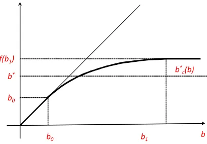
5.1.1 Characterization of the function b∗c(b)
The functionb∗
c(b) tells us, for any given initialb, the debt level that the mwc will choose when
it provides pork. To understand whatb∗
c(b) is, it isfirst useful to understand what it cannot be.
Suppose that the expected value functionEvc(b, A0) were strictly concave (as is the case without
a BBR). Then the objective function of the maximization problem in (12) would also be strictly
concave and there would be a uniquebb such thatb∗
c(b) = min{bb, b}. Thus, for any b larger than
bb, whenever the mwc chooses to provide pork, it would choose the debt levelbb. If this were the
case, however, a contradiction would emerge. To see why, note that for initial debt levelsbbelow
bb, the BBR would always be binding so that b0
c(b, A) =b for all A. On the other hand, for debt
levels abovebb, there will be statesA in which the BBR will not bind so thatb0
c(b, A)< b. This
means that whenbis belowbb, a marginal reduction of debt would be permanent: all future mwcs
would reduce debt by the same amount. By contrast, forbabovebb, a marginal reduction in debt
would have an impact on the following period, but it would affect the remaining periods only in
the states in which the BBR is binding. Indeed, when the BBR is not binding,b∗c(b) would equal
bb, and so would be independent ofb. It follows that the marginal benefit of reducing debt to the
left ofbbwould be higher than the marginal benefit of decreasing debt to the right ofbb. But this
contradicts the assumption that the expected value functionEvc(b, A0) is strictly concave.
The essential problem with a b∗
c(b) function of the form min{bb, b}is that the marginal effect
ofb onb∗
c(b) changes too abruptly atbb, from one to zero. In equilibrium, the debt level the mwc
chooses when it provides pork and the BBR is not binding must change more smoothly. This is not
possible when the expected value function is strictly concave, because the maximization problem in
(12) has a unique solution which allows noflexibility in choosingb∗
c(b). If the equilibrium expected
value function is concave, therefore, it must be weakly concave. Weak concavity does not pose
the same problem since it allows for the possibility that there are a range of debt levels that solve
the maximization problem in (12). Suppose this is the case and letb0denote the smallest of these
andb1 the largest; that is,
b0= min arg max{
b0
q +δEvc(b
0, A0)}, (14)
and
b1= max arg max{
b0
q +δEvc(b
Then any point in [b0, b1] will solve the maximization problem in (12). If the initial debt level b
is smaller thanb0, then we must haveb∗c(b) =b. But if the initial debt levelbexceedsb0 then the
associatedb∗
c(b) could be any point in the interval [b0,min{b, b1}]. This extraflexibility suggests
that there may exist a functionb∗
c(b) which guarantees that the expected value function is indeed
weakly concave. Fortunately, this is not only the case, but there exists a unique such function.
To make all this more precise, define an equilibrium under a strict BBR to be well-behaved
if (i) the expected value function is concave and differentiable everywhere, and (ii) the function
b∗c(b) is non-decreasing and differentiable everywhere. In addition, let (τb(A), gb(A)) be the tax
rate and public good level that solve the static maximization problem
max
(τ,g)
½
u(τ) +Alng+B(τ, g, b, b)
n :B(τ, g, b, b)≥0 ¾
. (16)
Then we have:
Proposition 4. There exists a unique well-behaved equilibrium under a strict BBR. The associated
function b∗
c(b)is given by:
b∗c(b) =
⎧ ⎪ ⎪ ⎪ ⎪ ⎪ ⎪ ⎨ ⎪ ⎪ ⎪ ⎪ ⎪ ⎪ ⎩
b0 ifb≤b0
f(b) ifb∈(b0, b1)
f(b1) ifb≥b1
, (17)
where the point b0 solves the equation
G(A∗(b0, b0)) +
Z A
A∗(b0,b0) µ
1−τb0(A) 1−τb0(A)(1 +ε)
dG(A) = n
q, (18)
the function f(b)solves the differential equation
n
q =G(A∗(b, f(b)))
h
1−dfdb(b)δ
³
1−n q
´i
+(nq)(1−δ)G(A∗(b, b))−(qn)G(A∗(b, f(b))) +RAA∗(b,b) ³
1−τb(A)
1−τb(A)(1+ε) ´
dG(A)(1−δ) +δnq
(19)
with initial condition f(b0) =b0, and the point b1 solves the equation
n
q(1−δ) = n
q(1−δ)G(A
∗(b
1, b1))−
µ n q −1
G(A∗(b1, f(b1))) +
Z A
A∗(b1,b1) µ
1−τb1(A) 1−τb1(A)(1 +ε)
dG(A)(1−δ).
(20)
The function b∗c(b) is tied down by the requirement that the objective function in the maxi-mization problem (12) must be constant on the interval [b0, b1]. In a well-behaved equilibrium,
this implies that −δE∂vc(b0, A0)/∂b0 = 1/q. Since the derivative of the expected value function
depends upon the functionb∗
c(b) and its derivative, this implies thatb∗c(b) satisfies a differential
equation with appropriate end-point conditions. This differential equation and its end-points are
spelled out in Proposition 4 and derived in its proof.
Figure 5 illustrates the equilibrium functionb∗
c(b). Thefigure highlights two key properties of
this function that will govern the dynamic behavior of the equilibrium. Thefirst property is that
b0 is strictly less than the level of debt that is chosen by the mwc when it provides pork in the
unconstrained case (i.e., b∗). This is immediate from a comparison of (10) and (18). The second
is that for any initial debt levelb larger thanb0,b∗c(b) is less thanb. This follows from the facts
thatb∗
c(b0) =b0anddbc∗(b)/dbis less than 1 forblarger than b0.
b0
b0
b*
f(b1)
b1 b
[image:27.612.202.406.363.505.2]b* c(b)
Figure 5: The lower bound b∗
c(b).
5.1.2 Dynamics and steady state
We now turn to the dynamics. Since in the unconstrained equilibrium, debt must lie in the interval
[b∗, b), we assume that when the BBR is imposed the initial debt level is in this range. We now
have:
Proposition 5. Suppose that a strict BBR is imposed on the economy when the debt level is in
the range[b∗, b). Then, in a well-behaved equilibrium, debt will converge monotonically to a steady
thanA∗(b0, b0), the tax rate will be τ∗, the public good level will be g∗(A), and a mwc of districts
will receive pork. When the value of the public good is greater thanA∗(b0, b0), the tax rate will be
τb0(A), the public good level will be gb0(A),and no districts will receive pork.
Proof: See Appendix.
To understand this result, note first from Propositions 3 and 4 that b0
c(b0, A) = b0 for allA
so thatb0 is a steady state. The key step is therefore to show that the equilibrium level of debt
must converge down to the level b0. Since debt can never increase, this requires ruling out the
possibility that debt gets “stuck” before it gets down to b0. This is done by showing that for
any debt level bgreater than b0, the probability that debt remains atb converges to zero as the
[image:28.612.211.391.335.506.2]number of periods goes to infinity.
Figure 6: Evolution of debt under a BBR
Figure 6 illustrates what happens to debt in the two shock case depicted in Figure 1. The
Figure depicts the two policy functions b0
c(b, AH) and b0c(b, AL). When the shock is high, the
constraint that debt cannot increase is binding and henceb0
c(b, AH) =bfor allb≥b0. When the
shock is low, however, the constraint is not binding and the mwc finds it optimal to pay down
debt. Given an initial debt level exceedingb∗, debt remains constant as long as the shock is high.
When the shock is low, debt starts to decrease. Once it has decreased, it can never go up because
of the BBR constraint. Debt converges down to the new steady state level ofb0.
policies in the unconstrained equilibrium.
Proposition 6. At the steady state debt level b0, the average primary surplus is lower than the
long run average primary surplus in the unconstrained equilibrium. In addition, the average level
of pork-barrel spending is higher.
Proof: See Appendix.
Recall that the primary surplus is the difference between tax revenues and public spending other
than interest payments. Thus, the first part of this result implies that steady state average tax
revenues must be lower under a BBR and/or average public spending must be higher. It should be
stressed, however, that this result only refers to the long run. In the transition to the new steady
state, at least initially, taxes will be higher and public good spending will be lower as revenues
are used to reduce debt.
The above analysis provides a reasonably complete picture of how imposing a BBR will impact
fiscal policy. However, we are also interested in the impact on citizens’ welfare. When it is first
imposed, it seems likely that a BBR will reduce contemporaneous utility. WhenAis low, instead
of transfers being paid out to the citizens, debt will be being paid down. When A is high, the
increase in taxes and reduction in public goods will be steeper than would be the case if the
government could borrow. Thus, in either case, citizen welfare should be lower. As debt falls, the
picture becomes less clear. On the one hand, citizens gain from the higher average public spending
levels and/or lower taxes resulting from the smaller debt service payments. On the other hand,
the government’s ability to smooth tax rates and public good levels by varying the debt level is
lost. Thus, there is a clear trade-offwhose resolution will depend on the parameters. The welfare
issue is therefore fundamentally a quantitative question and to resolve it we need to turn to the
calibrated model.
5.2
Quantitative analysis
The computation of the equilibrium is much easier with a strict BBR than without because the
function b∗
c(b) can be directly solved for. To see this, note that the steady state value of debt
b0 can be computed directly from equation (18), since the tax function τb(A) can be obtained
by solving the static problem (16). Given this, the function f(b) can be found immediately by
be found using equation (20).21 Once the functionb∗
c(b) is obtained, policy and value functions
can be computed following Step 2 in the algorithm described above (with the exception that the
constraint on debt is replaced byb0∈[b∗
c(b), b]). For the calibrated economy, wefind thatb0= 5.9,
a significantly lower value thanb∗, which was 29.4.
Table 3 compares fiscal policy variables in the steady state under a BBR with the long run
equilibrium values in the unconstrained case. The most striking difference is in the government
debt/GDP ratio which is reduced from 56.98% to 6.2% - a 89% decline. The steady state average
government revenue/GDP ratio is lower with a BBR and the mean government spending/GDP
ratio is higher. However, the variance of the government spending/GDP ratio is lower with a BBR
reflecting the fact that public good provision is less responsive to preference shocks. The variance
of tax rates is higher with a BBR, reflecting the intuition that taxes should be less smooth. In
the unconstrained case, the economy can have both responsive public good provision and smooth
taxes by varying debt. This is evidenced by the high variance of the debt/GDP ratio without a
BBR. The Table also shows that the average level of pork as a fraction of government spending
is considerably higher in the steady state under a BBR than in the long run in the unconstrained
case.22
GS/GDP GD/GDP GR/GDP=τ Pork/GS
Without BBR Mean 18.43% 56.98% 21% 0.015%
Stdev 5.40% 18.00% 1% 0.375%
With BBR Mean 19.45% 6.20% 19.78% 2.237%
[image:30.612.138.475.434.560.2]Stdev 2% 0.34% 2% 4.814%
Table 3: Long run effects of a BBR
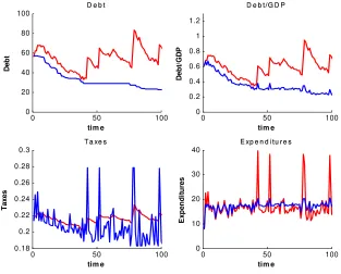
To understand the dynamic impact of imposing a BBR, we simulated the economy by drawing
a sequence of shocks consistent with our calibrated distribution ofA. As an initial condition, we
assumed that the government debt/GDP ratio equalled 63% which was the level prevailing in the
21
We use a fourth-order Runge-Kutta method to solve for the differential equation.
22
U.S. in 2005, the last year for which we have data. It took around 70 periods for the economy
to transition to a debt level belowb∗ (the equivalent of about a 30% debt/GDP ratio), with the
convergence to the new steady state (about a 6% debt/GDP ratio) occurring at a much slower
speed. Figure 7 compares the dynamics offiscal policy with and without a BBR. As can be seen
in thefirst panel of Figure 7, in the unconstrained case (the red line) the government always issues
debt in extraordinary times: with a BBR, however, it is forced to have zero deficits. This induces
a marked downward drift in the evolution of debt.
0 50 100
0 20 40 60 80 100 tim e De b t
D e b t
0 50 100
0 0.2 0.4 0.6 0.8 1 1.2 tim e De b t/ G DP
D e b t / G D P
0 50 100
0.18 0.2 0.22 0.24 0.26 0.28 0.3 tim e T axe s
T a xe s
0 50 100
0 10 20 30 40 tim e E x pe ndi tur e s
[image:31.612.146.459.273.525.2]E xp e n d i t u r e s
Figure 7: Evolution of key variables (- - red benchmark, — blue BBR )
The second panel of Figure 7 measures the debt/GDP ratio. Note that this measure spikes
during extraordinary times even with a BBR. The reason is that, even though debt remains
constant, GDP goes down due to the increase in taxation needed tofinance the war. The spike in
taxes during extraordinary times under a BBR is clearly illustrated in the third panel of Figure
7 which nicely illustrates the negative consequences of a BBR for tax smoothing. On the other