Classification of competitiveness types using copula

Munich Personal RePEc Archive

Classification of competitiveness types

using copula

Mereuta, Cezar and Albu, Lucian-Liviu and Ciuiu, Daniel

Romanian Center for Economic Modeling, Romanian Institute for

Economic Forecasting, Technical University of Civil Engineering,

Bucharest, Romania; Romanian Institute for Economic Forecasting

October 2010

Online at

https://mpra.ub.uni-muenchen.de/30430/

Classification of competitiveness types using copula

Cezar Mereuţă

Romanian Center for Economic Modeling (CERME), Bucharest, Romania e-mail: [email protected]

Lucian Liviu Albu

Romanian Institute for Economic Forecasting e-mail: [email protected]

Daniel Ciuiu

Technical University of Civil Engineering, Bucharest; Romanian Institute for Economic Forecasting

e-mail: [email protected]

Abstract

In this paper we classify competitive markets using a new form of normalized Herfindahl index and the degree of dominance of the leader. For this purpose we use the notion of copula, which connects two or more random variables with given marginals.

The parameters of the two marginals (which are supposed to be normal) are estimated by the moments' method, and the parameter of the copula is computed using the value τ of Kendall.

1. Introduction

In [7] there is defined the market share of the company i by the formula

T i

j n

j i i

CA CA

CA CA

Cp =

∑ =

=1

, (1)

where CA_i is the benefit of the company i. We denote next by p_i =Cp_i, and we reorder the companies such that p₁≥...≥ p_n. In this case p₁ is the weight of the leader (see [7]).

The Herfindahl index, or the informational energy of Onicescu is (see [9,10,7,11])

2 1

i n

i p

H

∑

=

= . (2)

In [7] there are considered 553 clustered markets, 235 in 2004 and 318 in 2008 as follows 1) In the year 2004:

a) 174 markets clustered CAEN Rev. 1 at group level (three digits) b) 47 markets clustered CAEN Rev. 1 at division level (two digits)

c) 13 markets clustered CAEN Rev. 1 at section level (one alphabetic character) d) one national system

2) In the year 2008:

a) 218 markets clustered CAEN Rev. 2 at group level (three digits) b) 80 markets clustered CAEN Rev. 2 at division level (two digits)

c) 19 markets clustered CAEN Rev. 2 at section level (one alphabetic character) d) one national system

If we denote by n the number of companies and by p1 the weight of the leader we obtain the regression

_[

_]

_[

_]

_[

_]

016634 .

0 008147

. 0 016777

. 0

164457 .

0 log 163945 .

0 log

239375 .

1

logH = p₁ − n +

(3)

maximum and minimum is 832.2702) Mereuţă (see [7]) introduced the normalized Herfindahl index: n n H M ln ln ln +

= . (4)

The above cohesion measure is the normalized quadratic Rényi entropy, where the quadratic Rényi entropy is R=−lnH.

Another parameter used to measure the cohesion of the market shares is the degree of dominance of the leader (see [7])

n n H p Gdl 1 1 1 2 1 − −

= . (5)

Noticing that 0≤M ≤1 and 0≤Gdl≤1 Mereuţă defines the matrix of cohesion degrees. There are obtained nine regions of the unit square using the lines Gdl =0.4, Gdl =0.6, M =0.4 and M =0.6.

Definition 1 ([12,8,13]) A copula is a function C:

[ ]

0,1n →

[ ]

0,1 such that 1) If there exists i such that x_i =0 then C

(

x₁,...,x_n

)

=0.

2) If x_j =1 for all j≠i then C

(

x₁,...,x_n

)

=x_i.

3) C is increasing in each argument.

We have the following theorem (see [12,8,13]).

Theorem 1 (Sklar) Let X₁, X₂,..., X be random variables with the cumulative distribution _n functions F₁, F₂,..., F , and the common cdf _n H

(

x₁,...,x_n

) (

=P X₁≤x₁,...,X_n ≤x_n

)

. In this case there exists a copula C

(

u₁,...,u_n

)

such that H

(

x₁,...,x_n

)

=C

(

F₁

( )

x₁ ,...,F_n

( )

x_n

)

. The copula C is well

defined on the chartesian product of the images of the marginals F₁, F₂,..., F . _n

Definition 2 ([12,14,15]) If n=2 the copula C is Archimedean if C

( )

u,u <u for any u∈

( )

0,1

and C

(

C

( )

u,v,w

)

=C

(

u,C

( )

v,w

)

for any u,v,w∈

[ ]

0,1 . If n>2 the copula C is Archimedean if

there exists a n−1 Archimedean copula C and a ₁ 2−Archimedean copula C such that ₂

(

u un

)

C

(

C

(

u un

)

un

)

C ₁,..., = _{2 1 1},..., ₋₁ , .

Consider a function ϕ:

(

0,1

]

→R decreasing and convex with ϕ

( )

1 =0 and its pseudo-inverse

g (g

( )

y has the value x if there exists x such that ϕ

( )

x = y and 0 in the contrary case). We know (see [5,12]) that a copula C is Archimedean if and only if there exists a function ϕ as above such that for any x,y∈

[ ]

0,1 we have

C

( )

x,y =g

(

ϕ

( ) ( )

x +ϕ y

)

. (6) In [14,15] there are presented methods to simulate Archimedean copulas, and in [2] there are presented algorithms to simulate queueing systems with one channel with arrivals and services depending through copulas.

In [4] there are found analytical formulae for the copulas that connect the number of customers in a Gordon and Newell queueing network, and their corresponding Spearman ρ and Kendall τ . This value is (see [8]):

(

)(

)

(

)

(

(

)(

)

)

( )

, 1 1 4 .

4 0 0 1 0 1 0 1 0 1 0 2 1 2 1 2 1 2 1 2 dudv dudv v u C Y Y X X P Y Y X X P v C u C v u C ∂ ∂ ∂ ∂ ∂ ∂∂ − = − ∫∫ ⋅ ∫ ∫ = < − − − > − − = τ

Sometimes we need the overlay probabilities, and we need in this case the notion of co-copula (see [14])

(

,...,

)

(

1 ,...,1

)

1

1 1

1 = − − +

∑

− +

=

∗ _{u u C u u u n}

C _i

n

i n

n . (8)

having the marginals F₁,..., F_n and they are connected by the copula C, we have

H

(

x₁,...,x_n

)

= P

(

X₁≥ x₁,...,X_n ≥ x_n

)

=C∗

(

F₁

( )

x₁ ,...,F_n

( )

x_n

)

, (8’) where F_i

( )

x_i =1−F_i

( )

x_i .

2. The new matrix of cohesion degrees using isolines

In the matrix of cohesion degrees defined by Mereuţă (see [7]) the regions are separated by

α

=

X , or by Y =β . The regions created by these lines are

(

₍

)

₎

( )

_{( )}

⎩ ⎨ ⎧ − = ≥ = ≤ α α α α F X P F X P

1 , respectively (9)

(

₍

)

₎

( )

_{( )}

⎩ ⎨ ⎧ − = ≥ = ≤ β β β β G Y P G Y P

1 , (9’) where F and G are the marginals of the Gdl (first axis) and M (second axis). But they do not take into account on the relation between the random variables Gdl and M .

Suppose that the above random variables have normal marginals, as in [7], but they are connected by the copula C. The marginal parameters are estimated using the moments’ method, and the parameter θ of the copula C is estimated as follows.

First we estimate τ using the empirical probabilities in the above formula, and next we compute the last term: we find τ in function of θ. For instance, in the case of Farlie-Gumbel-Morgestern copula (see [8,12]) we find

9 2θ

τ = , and from here (10)

2 9τ

θ = . (10’)

For the Fréchet family the copula is a mixture between the upper Fréchet bound, min and the copula product (the independence case) with the weights θ, respectively 1−θ. Due to the fact that in the min case we have τ =1, and in the product case we have τ =0 we obtain

θ =τ. (11) When the copula is Archimedean and we know the function ϕ in (6) we use the variables change x=ϕ

( )

u and y=ϕ

( )

v , and finally we obtain

( ) ( )

(

)

(

g x y

)

2dxdy

0

0 0

0

4

1− ⋅ ′ +

= ϕ

_∫

ϕ

_∫

τ . (7’)

In the case of Clayton family we have

( )

(

θ θ

)

θ 1 1 ,v = u− +v− − − u

C . (12)

From ( )_{( )}u_v

v C u C ϕ ϕ ′ ′ = ∂ ∂ ∂ ∂

we obtain first ϕ′

( )

_u =−_u−θ−1_{, and from here}

( )

θ

ϕ u = u−θ −1, and (12’)

_g

( ) (

_w = θ_w+₁

)

−θ1_{. (12”)}

Using (7’) we obtain

2 + = θ θ

τ , and from here (13)

τ τ θ − ⋅ = 1 2

. (13’)

( )

( ) ⎟⎟ ⎠ ⎞ ⎜⎜ ⎝ ⎛ − + − − ⋅ − = − + −₋ − − 1 ln 1 , _θ θ θ θ θ θ e e e e e v u C v u v u

. (14)

We obtain also the copula Prod for θ =0 and the copula min for θ →∞. For θ →−∞ we obtain the lower Fréchet bound W.

From ( )_{( )}u_v

v C u C ϕ ϕ ′ ′ = ∂ ∂ ∂ ∂

we obtain first

( )

− ₋₁ − = ′ u u e e u θ θ θ

ϕ , and from here

( )

_u

e e

u _{− ⋅}

−

− −

= _θθ

ϕ

1 1

ln , and (14’)

( )

=−1ln

(

γ − +1

)

, γ = −θ −1

θ e where e

w

g w . (14”)

For this family we obtain

τ =1−4⋅I, where (15)

(

)

(

)

dx

x x x I + + + ⋅ + =

_∫

1 1 1 ln 1 ln 1 0 2 γ

γ . (15’)

In the case θ ≠0 we multiply the relation (18’) by ln2

(

1+γ

)

_{, and in the case} θ =γ =τ =₀ and _I = 1_{4 we compute}

( )

36 1

0 =

′

I using the Taylor series for ln

(

1+x

)

and ₁₊1_{x. We obtain the}

Cauchy problem

( )

( ( )) ( ) ( ) ( ) ( ) (( )( ))

( )

( )

⎪ ⎪ ⎩ ⎪⎪ ⎨ ⎧ = = ′ ≠ = ′ + + ⋅ ⋅ + + _{− +} + 0 36 4 1 4 1 4 1 1 ln 1 1 ln 2 1 1 1 ln 2 γ γ γ γ γ γ γ

γ γ forI

I I I I I I I I .

Because _I=1−₄τ _{we obtain the Cauchy problem}

( )

( ( )) ( ) ( ) ( ) ( ) ( ) (( ) ( ))

( )

( )

⎪ ⎪ ⎩ ⎪⎪ ⎨ ⎧ = − = ′ ≠ = ′ + + ⋅ − ⋅ + + _{− +} ⋅ + 0 0 9 0 0 1 1 ln 1 2 1 4 1 ln 2 4 1 ln γ γ τ τ γ τ γ τ γ τ τ γ τ γ τ

γ γτ for

.

Finally we take into account that γ

( )

θ =e−θ −1 and γ′

( )

τ =−e−θ ⋅θ′

( )

τ . We obtain

( )

_{( )}

( )

( )

⎪ ⎪ ⎩ ⎪⎪ ⎨ ⎧ = = ′ ≠ = ′ − ⋅ − + − ⋅ 0 0 9 0 0 1 4 2 4 1 2 θ θ τ τ θ θθ

τθ for

e

. (16)

The above Cauchy problem is solved using the Runge-Kutta method.

In the case of the Gumbel-Hougaard family (see [5,8,13]) we have for θ ≥1 and β =_θ1

( )

(

( ) ( )

)

β θ θ _v u e v u

C , = − −ln +−ln . (17) For θ =1 we obtain the copula Prod and for θ →∞ we obtain the copula min .

From ( )_{( )}u_v

v C u C ϕ ϕ ′ ′ = ∂ ∂ ∂ ∂

we obtain first ϕ′

( )

u =−θ(−ln_uu)θ−1, and from here

ϕ

( ) (

u = −lnu

)

θ, and (17’) g

( )

x =e−xβ. (17”)

For this family we obtain

θ

τ θ − = 1 1

. (18’)

The Gumbel-Barnett copula is

C

( )

u,v =u⋅v⋅e−(θ( )( )lnu lnv), with 0<θ ≤1. (19) We notice that we have also the copula product (independence) for θ →0.

From ( )_{( )v}u

v C u C ϕ ϕ ′ ′ = ∂ ∂∂ ∂

we obtain first

( )

u _u(1 1_lnu)

θ

ϕ′ =− ₋ , and from here

( )

(

)

θ θ

ϕ u = ln1− lnu , and (19’)

( )

θ

θx e e x g −

= 1 . (19”) Using (7’) we obtain

=− ⋅ <0

− ∞

∫

dx x e e x β β

τ . (20)

where β =_θ2_.

The Ali-Mikhail-Haq copula is

( )

(

u

)(

v

)

v u v u C − − − ⋅ = 1 1 1 ,

θ , with −1≤θ ≤1. (21)

We notice that we have the copula Prod (independence) for θ =0. From ( )_{( )v}u

v C u C ϕ ϕ ′ ′ = ∂ ∂∂ ∂

we obtain first ′

( )

u =−_u(1−1_{( )1−u)}

θ

ϕ , and from here

( )

⎟ ⎠ ⎞ ⎜ ⎝ ⎛ ₊ − ⋅ − = u

u θ θ

θ

ϕ ln 1 1

1

, and (21’)

( )

_{( )} θ θ θ ₋ − = ₋ x e x g 1 1

. (21”)

Using (7’) we obtain

(

) (

)

θ θ θ θ τ 3 2 3 1 ln 1 2 1 2 2 − − − −

= . (22)

In the above formula τ is increasing on θ, and we have τ

( )

−₁ = 5−8₃ln2 _and

( )

3 1 1 =

τ . If we know τ we obtain θ using the bisection method.

Definition 3 Let

(

X,Y

)

be a bi-variate random variable such that the random variables X and Y

are connected by the copula C .

The copula of non-overlay, non-overlay for

(

X,Y

)

is C₁₁

( )

u,v =C

( )

u,v . The copula of overlay, overlay for

(

X,Y

)

is C₀₀

( )

u,v =C∗

(

1−u,1−v

)

. The copula of non-overlay, overlay for

(

X,Y

)

is C₁₀

( )

u,v =u−C

( )

u,v . The copula of overlay, non-overlay for

(

X,Y

)

is C₀₁

( )

u,v =v−C

( )

u,v .

Remark 1 If the marginal distributions are uniform on

[ ]

0,1 then, if we denote by H the common cumulative distribution function, we have: C₁₁

( )

u,v =H

( )

u,v =P

(

X ≤u,Y ≤v

)

, C₀₀

( )

u,v =

( )

u v P

(

X u Y v

)

H , = ≥ , ≥ , C₁₀

( ) (

u,v =P X ≤u,Y ≥v

)

and C₀₁

( ) (

u,v =P X ≥u,Y ≤v

)

. For other

marginal distributions, F and respectively G , we have P

(

X ≤x,Y ≤ y

)

=C₁₁

(

F

( ) ( )

x,G y

)

,

(

X xY y

)

C

(

F

( ) ( )

x G y

)

P ≥ , ≥ = ₀₀ , , P

(

X ≤ x,Y ≥ y

)

=C₁₀

(

F

( ) ( )

x,G y

)

and P

(

X ≥ x,Y ≤ y

)

=

( ) ( )

(

F x G y

)

C₀₁ , .

( )

( )

( )

( )

⎪ ⎪ ⎩ ⎪ ⎪ ⎨ ⎧ = = = = j j j j v u C v u C v u C v u C α α α α , , , , 01 10 00 11

, where j=1,k (23)

The corresponding isolines in x, are built from the isolines in y u, such that v x=F−1

( )

u and

( )

v

F

y= −1 . These are the separators of the regions bordered by _i

n i X x , 1 min min =

= , _i

n i X x , 1 max max = = , i n i Y y , 1 min min =

= and _i

n i Y y , 1 max max =

= . The above regions have corresponding regions in the plane Ouv

in the box bordered by u_min =F

(

x_min

)

, u_max =F

(

x_max

)

, v_min =G

(

y_min

)

and v_max =G

(

y_max

)

.

3. Application

Consider the above 553 clustered markets (see [7]). We have Gdl_min =0.074, 9997

. 0 max =

Gdl , M_min =0.1954, 9769M_max =0. . In [7] the marginal distributions are considered normal. Using the moments method we obtain µˆ_Gdl =Gdl =0.47432, σˆ_Gdl2 =S_Gdl2 =0.05801,

51181 . 0 ˆ_M =M =

µ and σˆ_M2 = S_M2 =0.01745. From these estimated parameters we obtain the box in the plane Ouv u_min =0.0067, 9988u_max =0. , v_min =0.0002 and v_max =0.9989.

The Kendal τ is 539860. . The parameter θ depending on the copula family is as in the following table.

Table 1: The value of the estimated parameter θ depending on the copula family.

Family Constraints on τ∈

[ ]

−1,1 θ

Clayton: θ >0 τ >0 346462. Frank: 0θ ≠ τ ≠0 009480. Gumbel-Hougaard: θ ≥1 τ ≥0 173232. Gumbel-Barnett: 10<θ≤ τ <0 not our case Ali-Mikhail-Haq: −1≤θ≤1 ₃1

3 2 ln 8

5− ≤τ ≤ _{not our case}

FGM: −1≤θ ≤1 τ ≤ ₉2 _{not our case} Fréchet: θ ≥0 τ >0 0.53986

In the following graphics there are represented first the above boxes in Ouv and Oxy , and the data points with U_i =F

(

Gdl_i

)

and V_i =G

( )

M_i , respectively X_i =Gdl_i and Y_i =M_i . We represent also the isolines (23) in the plane Ouv with k =2, α₁=0.4 and α₂ =0.6, and the corresponding isolines for the plane Oxy. These graphics are represented for each case of copula for which we have estimated the parameter θ (the constraints for the above tables are fulfilled).

In these graphics each class has a code given by four integer numbers: first number is for C00, the second number is for C01, the third number is for C10 and the last number is for C11. The number corresponding to a copula type depends on the position of its value and α_i, tackingα₀ =0 and α₃ =1. For instance the code from the fourth position is k if α_k ≤C₁₁

( )

u,v <α_k+1 for any u, v

[image:8.612.145.496.109.375.2]

for this class, and we memorize its class’s code if the point is in a new class. In each of the obtained regions we write the class number, and, between parentheses, the number of clustered markets from the involved class.

Fig. 1a: The graphics in the coordinates u, v in the case of Clayton copula

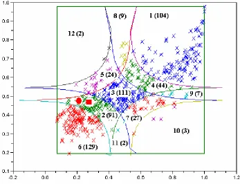
[image:8.612.144.492.417.681.2]

[image:9.612.144.494.97.366.2]

Fig. 2a: The graphics in the coordinates u, v in the case of Frank copula

[image:9.612.147.494.410.676.2]

[image:10.612.144.495.69.336.2]

Fig. 3a: The graphics in the coordinates u, v in the case of Gumbel-Hougaard copula

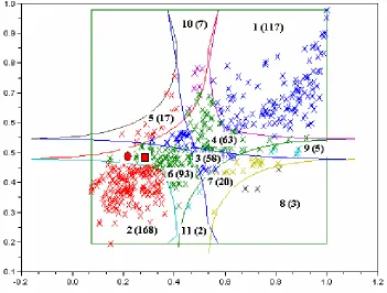
[image:10.612.143.497.378.645.2]

[image:11.612.141.495.56.325.2]

Fig. 4a: The graphics in the coordinates u, v in the case of Fréchet copula

Fig. 4b: The graphics in the coordinates x, y in the case of Fréchet copula

We notice that the two national systems from 2004 (represented by a circle in the above graphics, with Gdl=0.2287, M =0.4996, U =F

( )

Gdl =0.1524 and V =G

( )

M =0.4579) and 2008 (represented by a square in the above graphics, with Gdl =0.2861, M =0.4856,

( )

=0.2161

=F Gdl

[image:11.612.142.493.371.637.2]

(

,

)

0.6 4

.

0 ≤C₀₀ U V < , C₁₁

(

U,V

)

<0.4, C₀₁

(

U,V

)

<0.4, C₁₀

(

U,V

)

<0.4.

The numbers of clustered markets in each class depending on the year (2004, 2008 or both) and on the level (group, division, section or all three levels) are listed in Appendix A. The line of the class that contains the two national systems is bolded. The star at the exponent at “Total” means that the total does not contain the national system. Two stars in the last total means that we did not take into account the two national systems. For instance, in the case of Clayton copula the totals are 44* for the year 2004, 53* for the year 2008 and 97** for both year. It means that, if we take into account the national systems, these totals would be 45 for the year 2004, 54 for the year 2008 and 99 for both years.

4. Conclusions

Our classification has a probabilistic interpretation: each region obtained by isolines is such that the four probabilities resulting from the four copula types from definition 3 are in given intervals bordered by α_j. It has also more possible classes than the nine regions from the case of Mereuţă (see [7]): in each case of copula family there are 13 possible classes. Even the effective number of classes is greater (11 in the cases of Clayton and Fréchet copula, respectively 12 in the cases of Frank and Gumbel-Hougaard copula).

There are also similitudes between the classification of Mereuţă and those from this paper. In the classification of Mereuţă the regions with small Gdl and M, and with both values big (the heads of the main diagonal) there are relative big numbers of the contained clustered markets: both numbers are equal to 97. The same thing we can say about our case. For the smallest values of Gdl

and M we obtain 180 clustered markets in the case of Clayton copula, 129 clustered markets in the case of Frank copula, 170 clustered markets in the case of Gumbel-Hougaard copula, respectively 168 clustered markets in the case of Fréchet copula. For the highest values of Gdl and M we obtain 114 clustered markets in the case of Clayton copula, 104 clustered markets in the case of Frank copula, 126 clustered markets in the case of Gumbel-Hougaard copula, respectively 117 clustered markets in the case of Fréchet copula.

On the secondary diagonal the above numbers are small. The number of clustered markets with high Gdl and low M (the class from bottom-right corner) is 2 in the case of Mereuţă, respectively 3 in the case of this paper, for each case of copula.

The number of clustered markets with low Gdl and high M (the class from top-left corner) is 5 in the case of Mereuţă, 2 in the case of Frank copula, and 0 (no clustered market in the class) in the other cases.

In the case of Frank copula there is also an interesting similitude between our classification and the classification of Mereuţă for the middle class (medium Gdl and M): the number of clustered markets is 110 in the case of Mereuţă, and 111 in our case.

References

[1] G. Dall' Aglio: ''Fréchet classes: the beginning'', in Advances in Probability Distributions with

Given Marginals. Beyond the Copulas, Eds. G. Dall' Aglio, S. Kotz and G. Salinetti, Kluwer

Academic Publishers, 1991, pg. 1-12.

[2] D. Ciuiu: ''Simulation Experiments on the Service Systems Using Arrivals and Services Depending Through Copulas'', Analele Universitatii Bucuresti, No. 1, 2005, pg. 17-30.

[3] D. Ciuiu: Sisteme si retele de servire, Matrix Rom, Bucuresti, 2009.

[4] D. Ciuiu: ''Gordon and Newell Queueing Networks and Copulas'', Yugoslav Journal of

Operations Research, Vol. 19, No. 1, 2009, pg. 101-112.

[5] C. Genest: ''Statistical Inference Procedures for Bivariate Archimedean Copulas'', Journal of

American Statistical Association, Vol. 88, No. 423, 1993, pg. 1034-1043.

[6] S. Kotz, J.P. Seeger: ''A new approach to dependence in multivariate distributions'', in

Dall' Aglio, S. Kotz and G. Salinetti, Kluwer Academic Publishers, 1991, pg. 113-127.

[7] C. Mereuţă: Particularitati ale repartitiilor cotelor de piata ale companiilor active pe pietele

clasificate, din perspectiva gradelor de concentrare, Working Papers of Macroeconomic

Modeling Seminar, No. 102301, 2009, pp. 1-26.

[8] R. Nelsen: ''Copulas and association'', in Advances in Probability Distributions with Given

Marginals. Beyond the Copulas, Eds. G. Dall' Aglio, S. Kotz and G. Salinetti, Kluwer

Academic Publishers, 1991, pg. 51-74.

[9] O. Onicescu: ''Th eorie de l'information. Energie informationnelle'', C.R. Acad. Sci., Paris,

Serie A, 26, 263, 1966, pg. 841-842.

[10] O. Onicescu, V. Ştefănescu: Elemente de statistică informationala şi aplicaţii, Ed. Tehnică, Bucureşti, 1979.

[11] I. Petrică, V. Ştefănescu: Aspecte noi ale teoriei informaţiei, Ed. Academiei, Bucureşti, 1982. [12] E. Sungur and Y. Tuncer: ''The Use of Copulas to Generate New Multivariate Distributions'',

The Frontiers of Statistical Computation, Simulation & Modeling. Volume I of the Proceedings of the ICOSCO-I Conference (The First International Conference on Statistical

Computing, Çeşme, Izmir, Turcia, 1987, pg. 197-222.

[13] B. Schweizer: ''Thirty years of copulas'', in Advances in Probability Distributions with Given

Marginals. Beyond the Copulas, Eds. G. Dall' Aglio, S. Kotz and G. Salinetti, Kluwer

Academic Publishers, 1991, pg. 13-50.

[14] I. Văduva: Fast Algorithms for Computer Generation of Random Vectors used in Reliability

and Applications, Preprint nr. 1603, ian. 1994, TH-Darmstadt.

Appendix A

[image:14.612.50.571.115.295.2]

The numbers of clustered markets depending on the year and on the level

Table 2: The number of clustered markets in the case of Clayton copula

2004 2008 2004 and 2008

Class

number Group level

Division level

Section level Total

Group level

Division level

Section level Total

Group level

Division level

Section level Total

1 37 7 2 46 53 12 3 68 90 19 5 114

2 51 20 5 76 64 32 8 104 115 52 13 180

3 37 6 1 44* 37 10 6 53* 74 16 7 97**

4 27 7 1 35 26 13 1 40 53 20 2 75

5 2 2 1 5 5 3 1 9 7 5 2 14

6 9 3 2 14 17 6 0 23 26 9 2 37

7 6 1 0 7 9 2 0 11 15 3 0 18

8 2 0 0 2 1 0 0 1 3 0 0 3

9 1 0 0 1 4 1 0 5 5 1 0 6

10 1 1 1 3 2 1 0 3 3 2 1 6

[image:14.612.72.542.327.530.2]

11 1 0 0 1 0 0 0 0 1 0 0 1

Table 3: The number of clustered markets in the case of Frank copula

2004 2008 2004 and 2008

Class numb er Grou p level Divisio n level Sectio n level Tota l Grou p level Divisio n level Sectio n level Tota l Grou p level Divisio n level Sectio n level Tota l 1 31 7 2 40 49 12 3 64 80 19 5 104

2 32 11 2 45* 26 16 2 44* 58 27 4 89**

3 35 8 1 44 48 16 3 67 83 24 4 111 4 19 5 1 25 14 5 0 19 33 10 1 44

5 5 2 2 9 8 4 3 15 13 6 5 24

6 35 12 4 51 49 21 8 78 84 33 12 129

7 9 1 0 10 14 3 0 17 23 4 0 27

8 3 1 1 5 3 1 0 4 6 2 1 9

9 2 0 0 2 4 1 0 5 6 1 0 7

10 2 0 0 2 1 0 0 1 3 0 0 3

11 1 0 0 1 1 0 0 1 2 0 0 2

12 0 0 0 0 1 1 0 2 1 1 0 2

Table 4: The number of clustered markets in the case of Gumbel-Hougaard copula

2004 2008 2004 and 2008

Class numb er Grou p level Divisio n level Sectio n level Tota l Grou p level Divisio n level Sectio n level Tota l Grou p level Divisio n level Sectio n level Tota l 1 42 10 2 54 56 13 3 72 98 23 5 126

2 49 19 5 73 61 28 8 97 110 47 13 170

3 36 6 1 43* 35 13 6 54* 71 19 7 97**

4 23 4 1 28 25 12 1 38 48 16 2 66

5 2 2 1 5 5 3 1 9 7 5 2 14

6 11 4 2 17 18 7 0 25 29 11 2 42

7 6 1 0 7 8 2 0 10 14 3 0 17

8 2 0 0 2 1 0 0 1 3 0 0 3

[image:14.612.74.543.565.729.2]

10 1 1 1 3 2 1 0 3 3 2 1 6

11 1 0 0 1 1 0 0 1 2 0 0 2

[image:15.612.69.545.53.93.2]

12 0 0 0 0 1 0 0 1 1 0 0 1

Table 5: The number of clustered markets in the case of Fréchet copula

2004 2008 2004 and 2008

Class

number Group level

Division level

Section level Total

Group level

Division level

Section level Total

Group level

Division level

Section level Total

1 37 7 2 46 55 13 3 71 92 20 5 117

2 49 19 5 73 59 28 8 95 108 47 13 168

3 18 6 2 26 23 9 0 32 41 15 2 58

4 25 6 1 32 22 8 1 31 47 14 2 63

5 2 2 1 5 7 4 1 12 9 6 2 17

6 31 5 1 37* 35 13 6 54* 66 18 7 91**

7 6 1 0 7 10 3 0 13 16 4 0 20

8 2 0 0 2 1 0 0 1 3 0 0 3

9 1 0 0 1 3 1 0 4 4 1 0 5

10 2 1 1 4 2 1 0 3 4 2 1 7