SELECTIVE CONSISTENCY MODEL ON MONGODB BIG DATA STORE

1217

IMPROVED SELF-ORGANIZING MAPS BASED ON

DISTANCE TRAVELLED BY NEURONS

1_{HICHAM OMARA,} 2_{MOHAMED LAZAAR,} 3_{YOUNESS TABII}

1_{Abdelmalak Essaadi University, Tetuan, Morocco.}

E-mail: [email protected]

,

,

ABSTRACT

The Self-Organizing Map (SOM) is a commonly algorithm used for visualizing and classification of datasets, due to its ability to project high-dimensional data in a lower dimension. However, certain topological constraints of the SOM are fixed before the learning phase; the appropriate number of neurons has a major influence on the classification accuracy. Many researchers have tried to deal with this problem. This paper presents a novel approach to improve SOM based on distance travelled by each neuron. This approach is testing on two different databases of breast cancer. The model will classify the input vectors into two classes of cancer type (benign and malignant); the result obtained shows amelioration compared to classical SOM; up to 2% of improvement in classification accuracy is observed. We can conclude that our approach seems an efficient method in medical applications and especially for the cancer classification.

Keywords: Self-Organizing Maps, Weighting Optimization, Classification, Cancer.

1. INTRODUCTION

Today, breast cancer is one of the most frequently seen cancer types and the leading cause of cancer death among women both in the developed and less developed world. It is estimated that worldwide over 508 000 women died in 2011 due to breast cancer [1]–[3]. Classifying breast cancer is, for doctors, a source of important information. This provides help to determine the prognosis and allows well suggest the appropriate treatment, and then improve breast cancer survival.

Recently, the neural network has become a powerful tool in the classification of cancer database, and help doctors to select the best treatment; this is done due to its ability to model complex nonlinear systems with significant variable interactions, and its ability to learn from experience. The knowledge gained from the learning experience is stored, and it’s used to make decisions about new entries. Practically, machine learning methods such as artificial neural networks, support vector machine, Bayesian belief network, decision trees, genetic algorithms, k-means, have become indispensable in medical applications including prediction and prognosis of cancer. In addition, most of these learning algorithms supervised belong to a specific category of classifiers that classify on the basis of conditional

probabilities or conditional decisions (in supervised learning the 'categories' called labels are known).

1218 rough set (RS) based SVM classifier model, they used RS to select features and remove the redundant; their accuracy rate is around 99.8% in average [10]. Akay used the SVM algorithm combined with Feature Selection to trait breast cancer problem, his accuracy rate is around of 99,51% for the SVM model that contains five features [12]. Murat and Ince were proposed an algorithm based on association rules (AR) to reduce the dimension of database to four dimensions and Neural Network to classify breast cancer; they obtained a classification rate equal to 95.6% [13]. Nguyen et al. were classified the database with a Random Forest classifier and feature selection technique, the classification accuracy resulted is around 99.8% [14].

In this paper, a classification is tested through both classical and proposed SOM algorithm to help in the diagnosis of breast cancer. The training algorithms are compared using accuracy and computing time. The aim of our study is to reduce the number of neuron in the map. Our neural network approach works well, in terms of accuracy and computing time and this will lead to automated medical diagnosis system for the particular disease. The rest of paper is organized as follows. In Section 2, we introduce the SOM and we describe a novel neural network that we have proposed. In section 3, we describe the two databases and the pre-process of data. In Section 4 we applied our model, and we discuss the result. In the final section, we draw our conclusion.

2. KOHONEN TOPOLOGICAL MAPS

2.1. Self-Organizing Maps

The self-organizing maps (SOM) as one type of the neural networks are commonly used for visualizing and clustering of multidimensional data[15], [16]. Due to his ability to project high-dimensional data in a lower dimension, the SOM is applied in various areas: medicine, financial, ecological, engineering, law enforcement, and other fields [15]–[19]. The SOM often consists of a regular grid of map units. Each unit is represented by a vector , , … , , where d is input vector dimension. The units are connected to adjacent ones by neighbourhood relation. The SOM is trained iteratively. At each training step, a sample vector S is randomly chosen from the input data set, a metric distance is computed for all weight vectors W to find the reference vector W that satisfies a minimum distance or maximum

similarity criterion following the equation 1. The neuron with the most similar weight vector to the input pattern is called the Best Matching Unit (BMU).

‖ ‖ (1)

where is the neurons number in the map in instant . The weights of the BMU and its neighbours are then adjusted towards the input pattern, following equation 2.

1 , ‖ ‖ (2)

One of the main parameters influencing the training process is the neighbourhood function , between the winner neuron and neighbour neuron . This function is positive and symmetric defines a distance-weighted model for adjusting neuron vectors. It can be calculated using the equation 3.

,

‖ ‖

2 (3)

where ‖ ‖ ≅ ‖ ‖ , and are positions of the BMU neuron on the Kohonen map. The function decreases monotonically with time. This function can introduces zones of influence around each winner neuron, the weightings of each neuron are changed, but the degree of change decreases with the distance on the map between the positions of neuron to neuron winner and to make updated. The conventional SOM learning algorithm can be explained using the Algorithm 1.

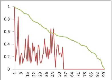
Figure 1: Normalised distance travelled by each neuron(green), and number of samples assigned to each

neuron (red line) 0

0.2 0.4 0.6 0.8 1

1219

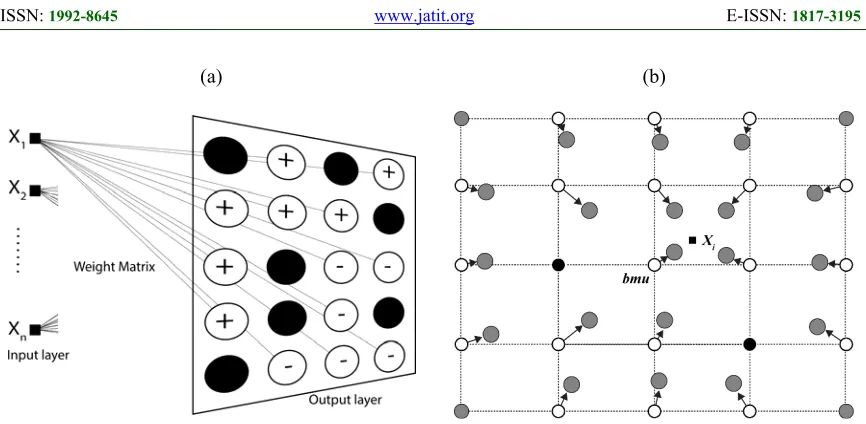
(a) (b)

Figure 2: (a): proposed SOM Representation (rectangular topology): The hidden layer is composed by the activated neurons (white circles: + represents benign tumour and - malignant one) and deactivated neurons (black circle). (b): Update BMU and its activated neighbours towards the input; the grey and white circles correspond to the situation

of neurons before and after; the black ones correspond to the deactivated neurons.

2.2. Proposed Self-Organizing Maps

In this work, we present an approach based on the distance travelled by each neuron to improve SOM; this approach was tested on WDBC and WBD to separate malignant from benign samples as illustrated in Figure 2. Our goal is to detect neurons

that have not made enough displacement during the first phase of learning (called deactivated neurons) and retrain the map just by the rest of neurons (activated neurons), so the size of the map will be reduced as well as the training time. The distance used in this study is the Euclidean distance defined as:

, (4)

Our algorithm is divided into two main steps. In the first, the network was trained by the classical SOM, in which we calculate the distance travelled by each neuron, and the data distribution into each neuron. The curve Figure 1 prove the result obtained; the green one shows the distance travelled by each neuron in the training phase and the red shows the number of neurons assigned to each neuron (called gain); this curve proves that if distance travelled decrease the gain increase, especially after the neuron 55 where no data has been assigned. Therefore we have noticed that from a large number of neurons at the beginning of the

algorithm, a few dozen contains the information, the others have no effect on the map. Then, we can remained just those neurons which their distance travelled are more than threshold (in this work the average was chosen). In the second phase, the card is retrained just with the active neurons using equation 2 as shown in Figure 2.

To do this, we have associated to each neuron a real number representing the distance it has travelled , with 1, … , . The value of di will be incremented by the distance travelled

by neuron i after each iteration during the first learning phase using equation 5.

1

, 1 (5)

In the end of the first step, the neuron that their distance is greater than average of distance travelled will be marked by 1 and the rest by 0.

1

(6)

Finally, we find a map that contains only the optimal neurons following equation 7.

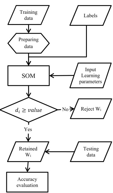
1220 Generally, neurons which their distance is less than a previously set value will be eliminated. The improved SOM learning algorithm can be explained in Figure 3.

Figure 3. Flowchart used in our model

3. EXPERIMENTAL

3.1. Database Description

The two Wisconsin Breast Cancer Datasets is provided by University of Wisconsin Hospitals, Madison, Wisconsin, USA by Dr. WIlliam H. Wolberg. A brief description of these datasets is presented in Table 1. Each dataset consist of some instances with a set of numerical features and each instance has one of two possible classes: benign or malignant.

3.1.1. Wisconsin breast cancer dataset

This databases WBD consists of 699 instances (458 or 65.5% instances are Benign and 241 or 34.5% instances are Malignant) and 11 attributes. These attributes are a unique

identification number, the class label that correspond to the type of breast cancer (benign or malignant), Clump Thickness, Uniformity of Cell Size, Uniformity of Cell Shape, Marginal Adhesion, Single Epithelial Cell Size, Bare Nuclei, Bland Chromatin, Normal Nucleoli and Mitoses. There are 16 instances where there is a single missing attribute. This dataset is available in [20].

3.1.2. Wisconsin diagnosis breast cancer

The Wisconsin Diagnostic Breast Cancer (WDBC) dataset consist of 569 instances (357 or 62,7% instances are benign and 212 or 37,25% instances are malignant) and 32 attributes; where the first two attributes correspond to a unique identification number and the diagnosis status (benign/malignant). The rest 30 features are computations for ten real-valued features, along with their mean, standard error and the mean of the three largest values (“worst” value) for each cell nucleus respectively. These ten real values are computed from a digitized image of a fine needle aspirate (FNA) of breast tumor, describing characteristics of the cell nuclei present in the image and are recorded with four significant digits. This dataset is available in [21].

Table 1: Description of Breast Cancer Datasets

Dataset _attributes N°. of _instances N°. of Class distribution

WBC 11 699 _{Malignant: 241} Benign: 458

WDBC 32 569 _{Malignant: 212} Benign: 357

3.2. Data Normalization

Normalization of data (all values in the dataset must take values in the range of 0 to 1) is an important step in data analysis [22]. Practice has shown that when the numerical input values are normalized, learning neural networks is often more efficient, leading to better classification and decision. Thus, normalizing entries in NNs can make learning faster. There are many types of standardization in the literature [23]; in this paper the min-max normalization technique was used (equation 7).

min

max min (8)

where , , min , max represents the value that should be normalized, normalized

Training

data Labels

Preparing data

SOM Learning Input parameters

Reject Wi

Testing data Retained

Wi

Accuracy evaluation

No

1221 value, minimum value of X, maximum value of X respectively.

3.3. Missing Values Replacement

Statistics suggest some approaches to address missing values in medical databases such as deleting all cases with missing values for the variables under consideration or replacing all missing values with means or median [11], [24]. We have chosen to fill the missing data by the median M following the equation (9) which divides the population studied in two groups containing the same number of individual. This is useful to give the breakdown of studied character, because about 50% of the study population has a term less than the median and 50% greater than the median modality.

2 , 2

, 1

2

(9)

where is the number of population studies.

3.4. Performance analysis

To evaluate proposed model, we used the classification accuracy . It is the number of correct predictions made divided by the total number of predictions made, multiplied by 100 to turn it into a percentage, which is computed by the equation 10. See [7] for more details.

100% (10)

where , represent the number of correctly classified samples and the total number of the samples, respectively.

4. RESULTS AND DISCUSSION

In our topology, the hidden layer consists of 100 neurons (10 10; the choice of the high number of neurons is to give more luck to all the neurons to contribute to the realization of the map. The output layer was determined by one neuron that can be benign or malignant as mentioned in Figure 2. The general algorithm of the proposed model is shown in Figure 3. Before the start of training process, dataset were loaded from the database, the missing values were replaced by median value, the data were normalized using min-max normalization

and all the weights has initialized to random numbers. When the training process is completed for the training data, the last weights of the network were saved to be ready for the testing procedure. The parameters was initialized as mentioned in Table 2 the output of the network was 0 for the class benign and 1 for the class malignant. The training algorithm used for this network is SOM following by proposed model. The testing process is done for the rest of samples. These samples are fed to the proposed network and it’s their output is recorded for calculation of the classification accuracy.

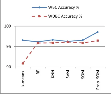
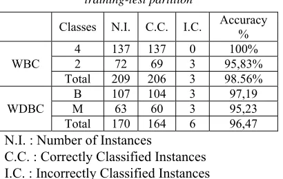
To illustrate the advantages of the proposed approach, we apply our algorithm to a widely used dataset, WDBC[21] and WBC[20]. The experiment results are presented in the Table 3. The accuracy was found to be equal 98.56% for WBC and 96,47% for WDBC. The comparison between proposed method and others ones by calculating the classification accuracy is tabulated in Table 5 and Figure 4. The results show that the proposed method gets a higher classification accuracy rate than the existing methods and up to 3% improvement over the conventional SOM. The number of neurons remaining in the maps after learning step presented in Table 4 (56 for WBC, 54 for WDBC) shows a precision when detecting the optimal number of neurons adapted for the map, and which automatically reduces the computation time. The threshold used is the average of the distance travelled. This choice is based on experience; we have tested other criteria like the middle and this threshold gives us the best result.

Figure 4: Comparison between proposed SOM and others methods with70–30% training-test partition

90 95 100

k‐

me

ans RF KNN SVM SO

M

Prop. SOM

WBC Accuracy %

1222

Table 2: Parameters used for SOM and Proposed SOM

Parameters Value

Number of input neurons 10×10 Learning rate 0.9

Radius 20

Distance Metric Euclidean Normalization attributes True

Initialization Random Sample

Number of iterations 1000

Table 3: Result obtained for proposed model by calculating the classification accuracy with 70–30%

training-test partition

Classes N.I. C.C. I.C. Accuracy _%

WBC

4 137 137 0 100% 2 72 69 3 95,83% Total 209 206 3 98.56%

WDBC

B 107 104 3 97,19 M 63 60 3 95,23 Total 170 164 6 96,47

N.I. : Number of Instances

C.C. : Correctly Classified Instances I.C. : Incorrectly Classified Instances

Table 4: Remained neurons in the maps

Initialized N° of neurons

Optimum N° of neurons

WBC 100 56

WDBC 100 54

Table 5: Classification accuracies obtained with our proposed system and other classifiers from literature for

70–30% training-test partition

Method _{Accuracy %} WBC _{Accuracy %} WDBC

k-means [25] _{(for k=5)} 96.56 _{(for k=5)} 90.86 Random Forrest

[26] 96.16 95.88 K-Nearest

Neighbor [27] (for k = 9) 96.65 (for k=7) 95.90 Support Vector

Machine [28] 96.27 96.12 SOM 96.56 95.88

Proposed method 98.56 96.47

5. CONCLUSIONS

We have proposed a modified learning algorithm of SOM, in which the optimal numbers of neuron are found by calculating their distances travelled in learning phase. The learning performance is then calculated using classification accuracy. The main innovation is to detect optimum neurons that can represent map with high accuracy. From a numerical point of view, the improved method gives better accuracy and low time for training, so reducing the size of the map and decreasing the memory size to store the map. The presented method considers the WBCD, and WBC, and can be extended to treat gene expression that contains thousands of features. The experimental results prove that the proposed SOM is better than the classical SOM. It can be concluded that our model gives fast and accurate classification and it works as a better tool for cancer classification.

Algorithm 1: Conventional self-organizing maps

α: learning rate

ρ: the radius of the neighbourhood function

for i=0 to maxIterations j ← InputVector(X); bmu ← select BMU(j,W);

Neighbours ← selectNeighbors(bmu,W,ρ);

foreach w ∊ Neighbours do

update w;

end for

α ← decrease Learning Rate(i,α); ρ ← decrease Neighborhood Size(i,ρ);

end for

Algorithm 2: Proposed self-organizing maps

α: learning rate

ρ: the radius of the neighborhoods function σ: mean of distance travelled

Savg : Standard-deviation of distance travelled

for i=0 to max_Iterations dist = 0 ;

j ← select Input Vector(X); bmu ← select BMU(j, W);

Neighbours←update Neighbours(bmu, W,ρ,σ,Savg);

foreach w ∊ Neighbors do

update (w);

update distance traveled by w;

end for

α←decrease Learning Rate(i,α); ρ←decrease Neighborhood Size(i,ρ);

1223

ACKNOWLEDGMENTS

The authors would like to thank the University of Wisconsin Hospitals, Madison; Dr. William H. Wolberg for providing the breast cancer dataset that was used in this work.

REFERENCES

[1] A. Jemal, F. Bray, M. M. Center, J. Ferlay, E. Ward, and D. Forman, “Global cancer statistics,” CA. Cancer J. Clin., vol. 61, no. 2, pp. 69–90, Apr. 2011.

[2] C. Jimenez-Johnson, “Understanding the Genetics of Breast Cancer: A Clinical Overview,” Internet J. Adv. Nurs. Pract., vol. 10, no. 1, Dec. 2008.

[3] H. Omara, M. Lazaar, and Y. Tabii, “Classification of Breast Cancer with Improved Self-Organizing Maps,” in Proceedings of the 2Nd International Conference on Big Data, Cloud and Applications, Tetouan, Morocco, 2017, p. 73:1–73:6.

[4] K. Polat and S. Güneş, “Breast cancer diagnosis using least square support vector machine,” Digit. Signal Process., vol. 17, no. 4, pp. 694– 701, Jul. 2007.

[5] E. D. Übeyli, “Implementing automated diagnostic systems for breast cancer detection,” Expert Syst. Appl., vol. 33, no. 4, pp. 1054– 1062, Nov. 2007.

[6] J. Joshi, R. Doshi, and J. Patel, “Diagnosis of Breast Cancer using Clustering Data Mining Approach,” Int. J. Comput. Appl., vol. 101, no. 10, pp. 13–17, Sep. 2014.

[7] L. Álvarez Menéndez, F. J. de Cos Juez, F. Sánchez Lasheras, and J. A. Álvarez Riesgo, “Artificial neural networks applied to cancer detection in a breast screening programme,” Math. Comput. Model., vol. 52, no. 7–8, pp. 983–991, Oct. 2010.

[8] A. M. Abdel-Zaher and A. M. Eldeib, “Breast cancer classification using deep belief networks,” Expert Syst. Appl., vol. 46, pp. 139– 144, Mar. 2016.

[9] A. Bhardwaj and A. Tiwari, “Breast cancer diagnosis using Genetically Optimized Neural Network model,” Expert Syst. Appl., vol. 42, no. 10, pp. 4611–4620, Jun. 2015.

[10] B. Zheng, S. W. Yoon, and S. S. Lam, “Breast cancer diagnosis based on feature extraction using a hybrid of K-means and support vector machine algorithms,” Expert Syst. Appl., vol. 41, no. 4, Part 1, pp. 1476–1482, Mar. 2014.

[11] A. M.Cedeño, J. Q.Domínguez, and D. Andina, “WBCD breast cancer database classification applying artificial metaplasticity neural network,” Expert Syst. Appl., vol. 38, no. 8, pp. 9573–9579, Aug. 2011.

[12] M. F. Akay, “Support vector machines combined with feature selection for breast cancer diagnosis,” Expert Syst. Appl., vol. 36, no. 2, Part 2, pp. 3240–3247, Mar. 2009. [13] K. Murat and M. C. Ince, “An expert system for

detection of breast cancer based on association rules and neural network,” Expert Syst. Appl., vol. 36, no. 2, Part 2, pp. 3465–3469, Mar. 2009.

[14] C. Nguyen, Y. Wang, and H. N. Nguyen, “Random forest classifier combined with feature selection for breast cancer diagnosis and prognostic,” J. Biomed. Sci. Eng., vol. 06, no. 05, p. 551, May 2013.

[15] T. Kohonen, “The self-organizing map,” Neurocomputing, vol. 21, no. 1, pp. 1–6, Nov. 1998.

[16] M. Ettaouil and M. Lazaar, “Vector Quantization by Improved Kohonen Algorithm,” J. Comput., vol. 4, no. 6, Jun. 2012. [17] I. Valova, G. Georgiev, N. Gueorguieva, and J. Olson, “Initialization Issues in Self-organizing Maps,” Procedia Comput. Sci., vol. 20, pp. 52– 57, Jan. 2013.

[18] S. Pavel and K. Olga, “Visual analysis of self-organizing maps,” Nonlinear Anal Model Control, vol. 16, no. 4, pp. 488–504, Dec. 2011. [19] M. Ettaouil, M. LAZAAR, and Y. Ghanou, “Architecture optimization model for the multilayer perceptron and clustering,” J. Theor. Appl. Inf. Technol., vol. 47, pp. 64–72, Jan. 2013.

[20] “UCI Machine Learning Repository: Breast Cancer Wisconsin (Original) Data Set.”

[Online]. Available:

https://archive.ics.uci.edu/ml/datasets/breast+ca ncer+wisconsin+(original).

[21] “UCI Machine Learning Repository: Breast Cancer Wisconsin (Diagnostic) Data Set.”

[Online]. Available:

https://archive.ics.uci.edu/ml/datasets/Breast+C ancer+Wisconsin+(Diagnostic).

[22] J. Sola and J. Sevilla, “Importance of input data normalization for the application of neural networks to complex industrial problems,” IEEE Trans. Nucl. Sci., vol. 44, no. 3, pp. 1464– 1468, Jun. 1997.

1224 Theory Eng., vol. 3, no. 1, pp. 89–93, Feb. 2011.

[24] C. M. Ennett, M. Frize, and C. R. Walker, “Influence of missing values on artificial neural network performance,” Stud. Health Technol. Inform., vol. 84, no. Pt 1, pp. 449–453, 2001. [25] J. A. Hartigan and M. A. Wong, “Algorithm AS

136: A K-Means Clustering Algorithm,” J. R. Stat. Soc. Ser. C Appl. Stat., vol. 28, no. 1, pp. 100–108, 1979.

[26] L. Breiman, “Random Forests,” Mach. Learn., vol. 45, no. 1, pp. 5–32, Oct. 2001.

[27] R. M. Parry et al., “k-Nearest neighbor models for microarray gene expression analysis and clinical outcome prediction,” Pharmacogenomics J., vol. 10, no. 4, pp. 292– 309, Aug. 2010.