Methods for the identification of asymmetric wavelets and factor analysis on the example of the monthly dynamics of the greenhouse gases of Antarctica

METHODS FOR THE IDENTIFICATION OF ASYMMETRIC WAVELETS AND FACTOR ANALYSIS ON

THE EXAMPLE OF THE MONTHLY DYNAMICS OF THE GREENHOUSE GASES OF ANTARCTICA

*Peter M. Mazurkin

Volga State Technological University, Yoshkar-Ola, Russia

ARTICLE INFO ABSTRACT

According to ESRL / GMD FTP data (as of March 9, 2017), regularities in the dynamics of the seven greenhouse gases of Antarctica at the SPO station since March 1975 were revealed and binary relations between them were obtained. In dynamics, as an influencing variable, we obtained a rating of CH4, CO, H2, C14C13, CO2, CO2O18, and CO2C13. Rating as dependent indicators starts with CH4, H2, CO. Greenhouse gas CO2 has the highest linear correlation coefficient of 0.9970. Its wavelet with a one-year cycle has a correlation coefficient of 0.8407. In Antarctica, due to the remoteness of the vegetation of South America and Australia, the semi-annual cycle is vague. However, this cycle is present elsewhere on the planet. With the highest correlation coefficient 0.7114 in Antarctica with a six-month cycle, CO is present, CH4 is in second place with 0.5626, and H2 is in third place with 0.3755. The main reason for the annual cycle is a change in the angle of inclination of the earth's axis. Even in Antarctica, the influence of this astronomical parameter on the fluctuation of greenhouse gases is noticeable. And semi-annual cycles depend, as a rule, on the vegetation cover of both hemispheres. Apparently, the semiannual cycles of CH4 and CH4CO13 can be explained mainly by the presence of ammonia reserves in Antarctica.

Copyright © 2019, Regiane Farias Camarão et al. This is an open access article distributed under the Creative Commons Attribution License, which permits unrestricted use, distribution, and reproduction in any medium, provided the original work is properly cited.

INTRODUCTION

To model the annual global carbon dynamics (Quéré et al., 2018) (in the Historical CO2 budget part of the Global Carbon Budget file), we used wave equations with variable amplitude and period of oscillation. The carbon budget largely depends on scenarios of greenhouse gas changes, which are considered in an article (Meinshausen et al., 2011) up to the year 2300. In the future, a factor analysis of the quantitative values of greenhouse gases in dynamics at different weather stations can be carried out. The relative contribution of various exposure factors varies over time, but most of the warming since 1891, as it turns out, is explained by the influence of a growing amount of greenhouse gases and anthropogenic aerosols (Folland et al., 2018). Global average surface temperatures rise in response to anthropogenic greenhouse gas emissions. The magnitude of this warming at equilibrium, called the specific equilibrium climate sensitivity, is still subject to uncertainty (Friedrich et al., 2016). Climate warming has led to the fact that photosynthetic absorption of carbon increases faster than its respiratory release from the terrestrial biosphere.

This increased the difference from summer to winter. Due to restrictions on carbon uptake by land vegetation, this negative feedback from warming in the boreal north and the Arctic cannot continue indefinitely (Forkel et al., 2016). Seasonal variations in atmospheric CO2 in the northern hemisphere have increased since the 1950s. This is due to an increase in seasonal CO2 exchange of approximately 50% in northern boreal forests (Graven et al., 2013). The newly developed concept is used to ensure that the negative greenhouse effect of the Antarctic Plateau is fully taken into account, indicating that it is controlled by vertical temperature changes and greenhouse gas absorption. The results show that the unique climatic conditions over the Antarctic plateau (strong surface temperature inversion and the deficit of free tropospheric water vapor) cause a negative greenhouse effect (Sejas et al., 2018). Then, to identify the patterns of negative greenhouse effect, in addition to the seven gases discussed in this article, it will be necessary to take into account temperature and water vapor.

Quantummeteorology: Quantization of data always occurs.

Even during the measurement process, quanta are determined by units. Especially quantization in meteorology occurs when

ISSN: 2230-9926

International Journal of Development Research

Vol. 09, Issue, 11, pp. 31081-31098, November, 2019

Article History:

Received xxxxxx, 2019 Received in revised form xxxxxxxx, 2019

Accepted xxxxxxxxx, 2019 Published online xxxxx, 2019

Article History:

Received 22nd _{August, 2019}

Received in revised form 13th _{September, 2019}

Accepted 16th _{October, 2019}

Published online 20th _{November, 2019}

Key Words:

Antarctica, gases, Relationships, Dynamics, Quanta, Wavelets.

*Corresponding author:Peter M. Mazurkin

RESEARCH ARTICLE

OPEN ACCESS

data is grouped, but earlier this was necessary to facilitate the process of manual processing of data series. Now, in the age of information technology, climatologists can abandon periodization and engage in the modeling of time series without their groupings. Of course, a heuristic interpretation is very necessary even a priori, but it should be carried out after processing the series of dynamics without grouping meteorological parameters. In the identification method, the series of meteorological data dynamics are modeled by a bundle of a large number of vibrations (Mazurkin, 2014, 2018), each of which has variable amplitudes and periods. Moreover, the oscillations can be infinite-dimensional in one direction or another from the beginning of the abscissa axis along the measurement time. Moreover, each fluctuation becomes a quantum of the indicator's behavior. Finite-dimensional wavelets are within a certain time interval and become solitons. A lot of vibrations form a certain integral bundle in the form of a strand of rope linked from many long and short threads. In dynamics, a trend is a special case of a wavelet with an extremely long oscillation period. As a result, the general statistical model of dynamics is a tourniquet linked from a set of particular equations of solitary waves (wavelets) with variable amplitude and period of oscillation. The proposed methodology for identifying nonlinear patterns (Mazurkin, 2014) makes it possible to distinguish dynamics waves from all measured and taken into account factors that can be further compared with heuristic representations of climate scientists. Therefore, the practical application of our methodology involves iterative identification, at least every year (and for monthly data, even every month). Moreover, each time an approximate forecast is made for the length of the forecast horizon equal to one third of the basis of the forecast. We believe that one of the conditions for the further development of meteorology is the identification of stable patterns (Mazurkin et al., 2018) from the accumulated series of statistical data, moreover, at each meteorological station. And these stable patterns will make it possible to better understand the past, while they are much more convenient to use in comparison with data tables. There are two types of quanta of behavior: firstly, in dynamics the factor is divided into the sum of wavelets, that is, in time the factor is represented as a bundle of solitary waves (solitons) and this identification process occurs as quantum certainty; secondly, the mutual influence of factors with a uniform or uneven measurement scale additionally receives quantum entanglement.

Method for identifying persistent patterns

The concept of modeling a statistical data sample: Statistical sampling is a multifactorial numerical field in the form of a

tabular model. By this definition, it differs from the tables of

statistical surveys. Moreover, not necessarily all the cells of the table must be filled. The tabular model may not have heuristic explanations. As a rule, authors of measurements, citing data tables in their publications, give a priori incorrect meaningful interpretations. This phenomenon of heuristic formalization is related to the fact that the table of measurement results, even if it is compiled correctly by the authors, cannot be consciously comprehended without conducting factor analysis with mathematical modeling of relationships between pairs of factors in the form of binary relationships. Then the tabular model (the initial numerical field) becomes the first, the quality of which is estimated by the error of the measurements, and the second in order is the desired complex algebraic equation (in the sense of Descartes),

composed of invariants (in the sense of Hilbert bricks). This process is statistical identification. The very unknown integral-differential equation becomes unnecessary, although, perhaps, someone will be able to get these integrals according to our models. At meteorological stations, many time series have been accumulated, for example, in Antarctica for several greenhouse gases. When identifying patterns in the article, ESRL / GMD FTP Data Finder data was used (as of March 9, 2017) at the SPO station (https://www.esrl.noaa.gov/ gmd/dv/data/index.php?site=spo&pageID=1&category=Green house%2BGases&frequency=Monthly%2BAverages&type=Fl ask).

We have adopted the following symbol conventions for greenhouse gases: CH4 – Methane; CH4C13 – C13/C12 inMethane; CO – CarbonMonoxide; CO2 – CarbonDioxide; CO2C13 – C13/C12 inCarbonDioxide; CO2O18 – O18/O16 inCarbonDioxide; H2 – MolecularHydrogen. For these gases, a common time scale was adopted from 03.1975 (





0

) in years (months are taken in fractions of a year)

Deterministicmodel

In general, the deterministic trend model contains the sum of two biotechnological laws (Mazurkin, 2014) in the form of an equation

2

1 т

т

т

у

у

y





, 2

exp(

4

)

3 1

1

a a

т

a

x

a

x

у





,

)

exp(

8 6 7 5 2 a a

т

a

x

a

x

у





, (1)

where

y

_т– trend,

x

– explanatory variable,

a

₁

...

a

₈ – model parameters (1).

Each parameter of model (1) has a physical meaning.

The general model (1) of the trend is not wave-like in two cases:

1) when the step of discrete measurements is too large compared to the period of vibrational disturbance of the measured real process (for example, the pulse of the electrocardiogram requires registration after 0.001 s);

2) when the interval of the measurement process is small compared to the half-period of the oscillatory perturbation of the measured parameter (for example, the average annual temperature at the point of the Earth requires registration for 100 years or more).

Asymmetric wavelet

We adhere to the concept of Descartes about the need to use a general algebraic equation as a finite mathematical solution of unknown integral equations. To generalize, a new class of wave functions has been proposed (Mazurkin, 2014). The conditions of existence in reality are most fully satisfied by the generalized asymmetric wavelet function of the form



  m i i y y 1

,

) ) exp( /( cos( )

exp( 3 5 6 8 10

1 9 7 4 2 i a i a i i a i a i

i a x a x x a a x a x a

y _ i _ i _{ } i _ i _

,

(2)

where

y

– indicator (dependent factor),

i

– number of the component (2),

m

– number of terms in the model (2), and the cosine is the connecting link between geometry and algebra,

x

– explanatory variable (influencing factor),

a

₁

...

a

₁₀ – parameters that take numerical values during structural-parametric identification of a mathematical construct (2).

In most cases, a truncated design (according to the formula for a half-period of oscillation) of an asymmetric wavelet of the type is sufficient to identify the desired patterns by known tabular models







m i i

y

y

1 ,

)

)

/(

cos(

)

exp(

_{3 5 6 8}

1 7 4 2 i a i i a i a i

i

a

x

a

x

x

a

a

x

a

y

_

i

_

i

_

_

i

_

. (3)

The number of model members in our examples reached 440 or more.

As a rule, the general stochastic wave function (3) has non-wave parts (1), which become special cases and show the deterministic behavior of the object of study in the measurement time interval. This allows you to identify the behavior of many mathematical, astronomical, biological and environmental, socio-economic and other objects (phenomena and processes) using composite statistical models.

Dynamic series of data as a sequence of signals

The physical and mathematical approach involves understanding the essence of a dynamic series of data as a reflection of a composite process or a variety of natural and / or natural and anthropogenic processes. For the first time, it was possible to obtain models of many series of dynamics up to the measurement error (Mazurkin, 2018; Mazurkin et al., 2018) by additively decomposing any dynamic series into many wavelet signals. A signal is a material storage medium. And we understand the information as a measure of

interaction. A signal may be generated, but its reception is

optional. For example, a number of primes has been known for several thousand years, but its essence as a set of signals has not yet been disclosed. A signal can be any physical process or part of it. It turns out that a change in the set of unknown signals has long been known, for example, through series of meteorological measurements at many points on the planet. However, theirstatisticalmodelshavenot vet beenobtained.

A wavelet signal, as a rule, of any nature (object of study) is mathematically written by the wave formula (Mazurkin, 2014) of the form

)

/

cos(

i 8i

i

i

A

x

p

a

y







, 2

exp(

4

)

3 1 i i a i a i

i

a

x

a

x

A





,

i

a i i

i

a

a

x

p

7

6 5





, (4)

where

y

– indicator (dependent factor),

i

– number of the model component (4),

m

– number of terms in the model (4),

x

– explanatory variable (influencing factor),

a

₁

...

a

₈ – model parameters (4) that take numerical values during semiautomatic structural and parametric identification in the

CurveExpert-1.40 software environment (URL: http://www.curveexpert.net/),

A

_i – the amplitude (half) of the

wavelet (axis

y

),

p

_i – half the oscillation period (axis

x

). According to formula (4) with two fundamental physical

constants (Napier number or time number) and (Archimedes

number or space number), a quantized wavelet signal is formed from the inside of the studied phenomenon and / or process. The concept of a wavelet signal allows us to abstract from the physical meaning of statistical series of measurements and consider their additive decomposition into components in the form of the sum of wavelets or behavior

quanta. The concept of an asymmetric wavelet signal or a

quantum of behavior (we do not consider the quantum of the structure of the object) allows us to abstract from the physical meaning of the dynamic series themselves (in the general case, not only dynamic ones) and consider their additive expansion in the form of the universal Descartes equation. Moreover, each quantum of behavior is characterized as a Hilbert brick, formed from the general equation of the wavelet signal (4).

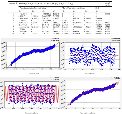
Patterns of dynamics CH4: Table 1 shows the values of the

model parameters (4). It can be seen from it that parts of the trend are special cases of the general wavelet signal.

As a rule, models of any dynamics (year, month, day, hours, minutes, seconds) by identification can be brought to a finite set of wavelet signals. The criterion for stopping identification is the measurement error, but for the year and month. Starting from adayorless, quantumentanglement appears between meteorological parameters. To reduce the volume of the article, for each of the seven greenhouse gases of Antarctica we present only the first 10 components. A negative sign in front of a component of the model indicates that increasing the value of this meteorological parameter is a crisis. The first term in the model (1) of the trend is the modified law of Laplace (in mathematics), Mandelbrot (in physics), Zipf-Pearl (in biology) and Pareto (in econometrics). It shows the exponential growth of CH4 over time.

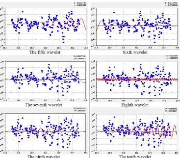
The first oscillation or the third term of the model with a correlation coefficient of 0.2621 shows some local behavior (a finite-dimensional wavelet signal). It may turn out that this is a process of humanity's awareness of the environmental situation due to the fact that this oscillation calms down, and in amplitude this wave of perturbation is eliminated over time. The pattern of CH4 dynamics over the months varies significantly with the advent of the second oscillation with a one-year cycle. The fourth member receives a correlation coefficient of 0.9747 for a cycle of one year. The influence of the inclination of the Earth's axis is significant, although the share of this influence is small compared to the trend. The fifth wavelet occurred during the measurement period from 02.1983 to 12.2015, and the sixth wavelet was in the past. The seventh wavelet is dangerous for the future, since it appeared around 2003 and began to increase in amplitude. The eighth wavelet with a six-month cycle apparently shows the influence of the ammonia deposit. The ninth and tenth wavelets were active in the past, they decrease in amplitude in the future.

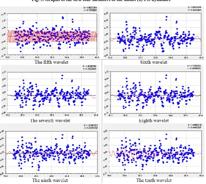
Patterns of dynamics CH4C13: This parameter of the

greenhouse gas system of Antarctica decreases with time (Table 2, Fig. 3). Four members of model (4) give a correlation coefficient of 0.9347. In a trend with an adequacy of 0.7860, the main influence is exerted by the second term according to the exponential growth law. As a result, there is a sharp decline. The third term decreases in amplitude and is an infinite-dimensional wavelet, and it is expelled after 2020. The next annual cycle increases in amplitude and also increases along the period of oscillation. The remaining six wavelets are graphically shown in Figure 4. The fifth, seventh and tenth members grow in amplitude in the future. The eighth term shows the increase with time of the amplitude and period of the six-month cycle of vibrational disturbance.

Patterns of dynamics CO: Carbon monoxide, unlike the two

[image:4.595.44.561.63.543.2]

previous gases, for the trend receives a correlation coefficient of only 0.1827 (Table 3, Fig. 5). Two conflicting forces affect CO growth.

Table 1. Dynamics model parametersСН4

Number i Wavelet 1 exp( 3 )cos( /( 5 6 ) 8 ) 7 4 2 i a i i a i a i

i a x a x x a a x a

y _ i _ i _{ } i _ Correl.

coeffic.

r

Amplitude (half) of the oscillation The half-period of oscillations Shift

i

a1 a2i a3i a4i a5i a6i a7i a8i

1 1472.4510 0 -3.52423e-5 2.28247 0 0 0 0 0.9990

2 8.90617 1.13936 0.00021773 2.53221 0 0 0 0

3 9.41014e-17 26.55429 7.56724 0.56482 3.71977 0.13669 0.56554 5.41199

4 13.43872 0 -0.0044830 1 0.49985 0 0 -0.52689

5 -4.06834e-5 5.61403 0.28040 0.99637 1.00176 0.0017977 1.59657 -0.23321 0.6409

6 -1.43777e9 0 17.48446 0.075291 3.30558 0 0 0.66131 0.2143

7 -4.55435e-36 30.61487 0.63190 1.05563 1.62402 0.00019604 1.59029 3.06517 0.3726

8 1.32689 0 0 0 0.24991 0 0 1.02523 0.5626

9 1.57774e6 0 12.17894 0.066124 0.71419 0.18769 0.18527 3.78512 0.3042 10 -0.11208 2.11835 0.39334 0.83085 1.10396 0.024370 1.03752 0.54151 0.2976

Two-term trend First oscillation

The second oscillation Trend and two oscillation

Fig. 1. Graphic dynamics of CH4: S - dispersion; r - correlation coefficient S = 11.39517168

r = 0.97758444

5.0 11.6 18.2 24.8 31.3 37.9 44.5

1530. 96 1580. 37 1629. 78 1679. 18 1728. 59 1778. 00 1827. 41

S = 11.01092162 r = 0.26212635

5.0 11.6 18.2 24.8 31.3 37.9 44.5

-26.94 -17.94 -8.94 0.06 9.06 18.06 27.06

S = 2.44733543 r = 0.97472060

5.0 11.6 18.2 24.8 31.3 37.9 44.5

-24.52 -16.76 -9.00 -1.24 6.52 14.28 22.04

S = 2.44237587 r = 0.99900228

5.0 11.6 18.2 24.8 31.3 37.9 44.5

1530.9 6 1580.3 7 1629.7 8 1679.1 8 1728.5 9 1778. 00 1827.4 1

According to the law of exponential growth, infinite-dimensional growth occurs according to the first term, but this is counteracted by a (negative sign) decrease according to the law of exponential growth. The influence of the annual cycle with a high correlation coefficient of 0.9389 with a slowly decreasing amplitude and an increasing frequency of vibrational disturbance immediately manifests itself.

The fourth wavelet with a correlation coefficient of 0.3396 will descend from the scene of the SPO weather station in the future. The overall adequacy is 0.9484. The CO dynamics is mainly influenced by the tilt of the Earth's axis. Figure 6 shows the graphs of the remaining six member of the general model (4). Of these, the fifth term with a constant six-month cycle with slowly decreasing amplitude is distinguished.

The fifth wavelet Sixth wavelet

The seventh wavelet Eighth wavelet

[image:5.595.47.559.46.518.2]

The ninth wavelet The tenth wavelet

Fig. 2. Charts of the remaining members of the model (4) CH4 dynamics

Table 2. Dynamics model parametersСН4c13

Numberi Wavelet 1 exp( 3 )cos( /( 5 6 ) 8 )

7 4 2 i a i i a i a i

i a x a x x a a x a

y _ i _ i _{ } i _ Correl. coeffic.

r

Amplitude (half) of the oscillation The half-period of oscillations Shift i

a1 a2i a3i a4i a5i a6i a7i a8i

1 -48.04243 0 0.0022232 0.99302 0 0 0 0 0.9347

2 -0.0067288 1.66351 0 0 0 0 0 0

3 5.53999e6 0 10.73974 0.16337 4.23608 0.37654 0.11239 -4.63300 4 -0.022092 0 -0.032033 0.99583 0.50117 8.23253e-6 1 -1.27097

5 -2.79984e-17 11.84452 0.15849 1.08983 5.23789 -0.056635 1.01107 -0.057671 0.4538 6 -1.08520 0 0.25005 0.84686 2.59160 -0.017996 1.02023 -1.13872 0.2754 7 -1.10809e-12 7.80598 0.11441 1.03617 3.83044 -0.0095556 1.03429 2.12313 0.2609 8 -0.0065997 0 0.0031710 1 0.24250 5.46935e-8 1 0.42400 0.1353 9 1.04641e-50 40.98792 0.24996 1.39125 0.84020 0.0040494 0.93121 2.89583 0.2531 10 8.83255e-13 8.42391 0.16930 1.00462 0.80669 -0.00016742 1.13116 -2.19305 0.4701

S = 1.85772329 r = 0.64093504

5.0 11.6 18.2 24.8 31.3 37.9 44.5

-7.67 -5.02 -2.37 0.28 2.94 5.59 8.24

S = 1.80742402 r = 0.21426030

5.0 11.6 18.2 24.8 31.3 37.9 44.5

-6.87 -4.64 -2.41 -0.17 2.06 4.29 6.53

S = 1.68375807 r = 0.37257031

5.0 11.6 18.2 24.8 31.3 37.9 44.5

-6.71 -4.48 -2.24 -0.00 2.23 4.47 6.71

S = 1.38289036 r = 0.56255773

5.0 11.6 18.2 24.8 31.3 37.9 44.5

-6.59 -4.60 -2.60 -0.61 1.38 3.38 5.37

S = 1.32373130 r = 0.30416262

5.0 11.6 18.2 24.8 31.3 37.9 44.5

-5.10 -3.45 -1.80 -0.16 1.49 3.13 4.78

S = 1.26472339 r = 0.29757976

5.0 11.6 18.2 24.8 31.3 37.9 44.5

[image:5.595.73.524.550.692.2]

[image:6.595.122.479.61.272.2]

Fig. 3. Charts of the first four members of the model (4) dynamics CH4C13

Fig. 4. Charts of the remaining members of the model (4) dynamics CH4C13

Table 3. Dynamics model parameters СO

Number

i

Wavelet 1 exp( 3 )cos( /( 5 6 ) 8 )

7 4

2

i a i i a

i a

i

i a x a x x a a x a

y _ i _ i _{ } i _

Correl. coeffic.

r

Amplitude (half) of the oscillation The half-period of oscillations Shift

i

a1 a2i a3i a4i a5i a6i a7i a8i

1 48.43987 0 -0.0075190 1.34737 0 0 0 0

0.9494

2 -0.023632 2.24414 0 0 0 0 0 0

3 13.20221 0 0.0044333 1 0.49967 -8.29847e-6 1 -0.51377

4 -2.12592 0 7.16563e-5 2.54239 1.02814 0.017815 0.97724 5.72490

5 3.78298 0 0.010130 1 0.24990 0 0 0.008918 0.7114

6 0.59175 0 -0.011475 1 1.49703 0 0 0.46960 0.3016

7 -0.18180 -0.0082160 1.39378 1.52419 0.0037388 1.02198 3.78710 0.1932 8 -5.77451e-8 5.88719 0.0024616 2.09674 -0.048959 0.36156 0.27699 5.00286 0.3995 9 0.00062055 2.76084 0.048218 1.11863 1.07816 -0.00062556 1.38097 -4.26084 0.3332 10 4.72631e-10 9.22795 0.15357 1.22451 0.32045 0.017037 0.74943 -4.08565 0.4405

[image:6.595.116.484.300.622.2]

Then it is clear that a decrease in the area of vegetation leads to a decrease in the content of CO in Antarctica. The sixth and seventh members show a slow, infinite-dimensional increase in amplitude, and the remaining wavelets in the near future will leave the territory of Antarctica at the SPO weather station.

Patterns of dynamics CO2: An article (Graven, 2013) states

that the annual cycle is associated with seasonal variations in CO2 due to boreal forests in the Northern Hemisphere.

[image:7.595.100.500.56.290.2]

We received annual and semi-annual CO2 cycles at Mauna Loa Hawaii Station in the Southern Hemisphere. According to the influence of external astronomical factors on the Earth’s climate (http://moodle.emaris.net/mod/page/view.php?id=19), the main reason for seasonality is a change in the angle of inclination of the earth's axis. For weather stations and forests, the angle of incidence of sunlight is also important. Then the annual cycle of greenhouse gases refers to the effect on the climate of the angle of inclination of the Earth's axis. And semi-annual cycles depend on the vital activity of the Fig. 5. Graphs of the first four members of the model (4) CO dynamics

[image:7.595.101.503.302.660.2]

vegetation cover of both hemispheres. As can be seen from table 4, seven wavelets are infinite-dimensional, and three (including the second term) are finite-dimensional (Fig. 7, Fig. 8).

[image:8.595.60.546.127.483.2]

Very high adequacy of 0.9994 for the trend. This explains the attention of scientists to this gas. The growth is explained by the second term according to the exponential law, although the natural first term shows a decrease in CO2 in amplitude.

Table 4. Dynamics model parameters СO2

Number i

Wavelet 1 exp( 3 )cos( /( 5 6 ) 8)

7 4

2

i a i i a

i a

i

i a x a x x a a x a

y _ i _ i _{ } i _

Correl. coeffic.

r

Amplitude (half) of the oscillation The half-period of oscillations Shift

i

a1 a2i a3i a4i a5i a6i a7i a8i

1 331.33275 0 0.00021991 2.04924 0 0 0 0

0.9997

2 0.47909 1.60522 0 0 0 0 0 0

3 1.12511 0 0.017117 1 9.47372 -6.66399e-6 2.28449 -2.14621

4 -1.33014 0 0.057150 1 74.66812 -67.57379 0.010273 0.11860

5 0.58293 0 0.00046085 1 0.49994 0 0 -0.19157 0.8407

6 6.57239e-17 0 -34.26893 0.0093099 8.94441 -5.59900 0.037018 -2.31213 0.3613

7 0.23526 0 0.011400 1 -0.027299 1.27556 0.093374 1.71229 0.5441

[image:8.595.133.472.498.797.2]

8 4.47699e-13 11.40992 0.12494 1.36849 1.00299 0.00074805 1.77357 0.07818 0.2955 9 0.32740 0.21503 0.37176 1 0.29983 -0.038784 0.46984 0.42914 0.1877 10 0.65207 0 1.30787 0.20937 0.31588 0.14398 0.044207 1.17841 0.2590

Fig. 7. Graphs of the first four members of the model (4) CO2 dynamics

Fig. 8. Charts of the remaining model members (4) CO2 dynamics

Table 5. Dynamics model parameters СO2C13

Number

i

Wavelet 1 exp( 3 )cos( /( 5 6 ) 8)

7 4

2

i a i i a

i a

i

i a x a x x a a x a

y _ i _ i _{ } i _

Correl. coeffic.

r

Amplitude (half) of the oscillation The half-period of oscillations Shift

i

a1 a2i a3i a4i a5i a6i a7i a8i

1 6.83282 0 -0.0038789 1.00679 0 0 0 0

0.9944

2 -0.047372 1.09347 0.049398 1.01029 0 0 0 0

3 -0.040142 0 0.34971 0.26635 0.12284 0.0098489 1.11036 1.57146 4 -0.00010278 0 -0.78668 0.51598 14.61623 -0.23503 1.00706 -1.83651

5 -5.10028e-23 18.08242 0.17626 1.30188 5.62235 -0.030756 1.23162 -0.59511 0.2935 6 -1.12347e-12 10.09309 0.36620 1.01215 1.37599 -0.0028025 1.01306 -5.13556 0.3627

7 -0.025851 0 0.015377 0.49296 0.50088 0 0 -0.14156 0.7886

8 1.01839e8 2.78657 1.59750 1.00425 1.14247 -0.00053606 1.14026 3.43409 0.3290 9 -5.62905e-8 5.34170 0.22298 1.00043 0.76509 -2.64366e-5 1.02439 -2.40669 0.4188

[image:9.595.43.548.81.755.2] [image:9.595.111.483.447.786.2]

10 -4.27359e-6 1.71976 0 0 2.67748 0.013525 1.03271 2.41098 0.1407

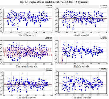
Fig. 9. Graphs of four model members (4) CO2C13 dynamics

Then it turns out that growth can mainly be explained by anthropogenic influence. The first wave occurs with an adequacy of 0.5020, and the second - 0.4539. Together, four members give 0.9997, that is, the increase from two fluctuations was only 0.9997 - 0.9994 = 0.0003. The set of oscillations during identification to the measurement error will give an increment of 1 - 0.9994 = 0.0006. The trend gets crucial importance and it becomes noticeable to everyone. The fifth term with a correlation coefficient of 0.8407 and a slowly decreasing amplitude shows the annual cycle of the influence of the tilt of the Earth's axis. The eighth wavelet shows a two-year cycle of plant productivity with a slight increase in the period. Vegetation changes the CO2 content in semi-annual cycles.

The temperature of the air on Earth changes similarly in cycles of six months. But a clear six-month cycle is not observed in Antarctica; wavelets with a changing period of six months are obtained. This is due to the distance from South America and Australia.

Patternsofdynamics CO2C13: A trend also has a strong

influence (Table 5, Fig. 9) with a correlation of 0.9919. The amplitude decreases, and the annual fluctuation due to the negative sign is directed against the growth of the indicator. The eighth wavelet shows that before the measurement period a strong unknown vibrational disturbance occurred.

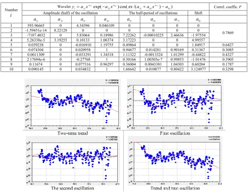
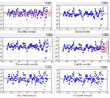
Patternsofdynamics CO2O18: The trend gives an average

level of adequacy with a correlation coefficient of 0.6104 (Table 6, Fig. 11). However, the fourcomponentsofmodel (4) gave a strongconnection. The annual cycle for the fifth component (Fig. 12) occurs with an increase in amplitude. Therefore, this cycle can become dangerous for the future. Due to the sharp increase in amplitude, the seventh and eighth wavelets, according to the law of exponential growth, also become dangerous for Antarctica. In this regard, even insignificant wavelets need to be analyzed for the future.

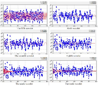
Patternsofdynamics H2: The trend (Table 7, Fig. 13) receives

a weak level of 0.3606. The first swing with a period of 4.4 years is 0.3816. The annual cycle at 0.8569 gives a strong adequacy.

[image:10.595.54.550.237.621.2]

Due to the negative sign in front of the fourth component, the influence of the tilt of the Earth's axis is directed against the growth of H2. As a result, four members give a correlation coefficient of 0.8987. At the same time, since January 2015, there has been a sharp decrease in H2. Re-identification of all greenhouse gases must be carried out with data up to the current month. Then there will be the possibility of forecasting for those wavelets that affect the future. affect the future.The seventh, eighth, and ninth wavelets with constant cycles become interesting: six-month, a cycle of 0.8 (three quarters) of a year, and a cycle of 0.33 or one third of a year. In this case, the seventh and eighth cycles act against the growth of greenhouse gas H2, and the ninth wavelet acts in the direction Table 6. Dynamics model parameters СO2O18

Number i

Wavelet 1 exp( 3 )cos( /( 5 6 ) 8 )

7 4

2

i a i i a

i a

i

i a x a x x a a x a

y _ i _ i _{ } i _

Correl. coeffic.

r

Amplitude (half) of the oscillation The half-period of oscillations Shift

i

a1 a2i a3i a4i a5i a6i a7i a8i

1 593.96665 0 4.34396 0.046109 0 0 0 0

0.7869

2 -1.59451e-14 8.22128 0 0 0 0 0 0

3 -7187.4032 0 5.83064 0.18986 7.22262 -0.00010225 2.46636 -1.97554

4 5.26338e-5 3.19255 0.10133 1.06374 3.17223 0 0 4.99557

5 0.039238 0 -0.016910 1.19755 0.49864 0 0 1.84917 0.6427

6 0.074304 0 0.020958 1 0.94677 0.014281 0.90169 0.31367 0.3085

7 0.0011309 0 -0.033291 1.34518 1.11322 -0.0013324 1.01299 -0.44822 0.4327 8 2.17694e-6 0 -0.27768 1 0.30166 1.00305e-7 0.99853 -1.01476 0.3903 9 0.11674 0 0.077316 0.96297 0.36004 0.0043381 1.04303 0.60204 0.1787

10 0.090145 0 0.034832 1 1.66642 0.010877 0.80422 3.124977 0.3298

Fig. 11. Charts of the first four members of the model (4) dynamics of CO2O18

[image:11.595.127.491.45.368.2]

[image:11.595.55.555.405.780.2]

Fig. 12. Charts of the remaining model members (4) CO2O18 dynamics

Table 7. Dynamicsmodelparameters Н2

Numberi

Wavelet 1 exp( 3 )cos( /( 5 6 ) 8)

7 4

2

i a i i a

i a

i

i a x a x x a a x a

y _ i _ i _{ } i _

Correl. coeffic.

r

Amplitude (half) of the oscillation The half-period of oscillations Shift

i

a1 a2i a3i a4i a5i a6i a7i a8i

1 443.77671 0 0.00010356 3.22277 0 0 0 0

0.8987

2 0.30402 2.90305 0.027663 1.31371 0 0 0 0

3 2.30564 0 -0.029504 1 2.20175 0 0 4.05771

4 -15.37557 0 0.019083 1 0.50130 0 0 -1.57910

5 7.57341 0 0.035090 1 1.65734 -0.0063322 1 -0.52453 0.5665

6 9.66598e-55 56.45861 2.11985 1.01677 1.54815 -0.0034306 1.43983 -1.93804 0.6253

7 -27971.382 0 7.69897 0.080775 0.25286 0 0 -3.37251 0.3755

8 -2.37529e8 0 11.40526 0.17045 0.40349 0 0 -1.50284 0.2600

9 0.59073 0 -0.00016459 2.50892 0.16735 0 0 1.12556 0.3267

10 1.96688e-21 17.44623 0.0030724 2.44393 2.50101 -0.58344 0.30958 -1.60554 0.3993

of this increase. Next, by factor analysis, we determine the significance of each of the gases.

Factor analysis of greenhouse gas trends: Table 8 shows the

correlation matrix of binary relationships and the rating of factors as influencing variables and as dependent indicators

[image:12.595.119.488.139.462.2]

obtained by the identification method (Mazurkin and Kudrjashova, 2018) for the seven greenhouse gases of Antarctica. In the diagonal cells there are also correlation coefficients of the trend, and relationships were revealed according to data from 01.1998 to 07.2015.

[image:12.595.69.534.508.631.2]

Fig. 14. Graphs of the remaining members of the model (4) dynamics H2

Table 8. The correlation matrix and ranking of factors by trend (1)

Influencing factors (parameterx)

Dependent factors (indicatory) Amountr Place x

I

CH4 CH4C13 CO CO2 CO2C13 CO2O18 H2

CH4 0.9776 0.7481 0.8110 0.3259 0.3755 0.1805 0.6215 4.0401 1 CH4C13 0.7481 0.7860 0.6705 0.0324 0.0090 0.3636 0.6170 3.2266 3 CO 0.8501 0.6967 0.1827 0.1960 0.2131 0.3925 0.7192 3.2503 2 CO2 0.4966 0.0324 0.0209 0.9994 0.9620 0.3889 0.3130 3.2132 4 CO2C13 0.3755 0.0090 0.0592 0.9620 0.9914 0.4197 0.2139 3.0307 5 CO2O18 0.2940 0.3875 0.3727 0.4376 0.4506 0.6104 0.3330 2.8858 7 H2 0.6110 0.6170 0.6431 0.3711 0.2139 0.1611 0.3606 2.9778 6 Amountr 4.3529 3.2767 2.7601 3.3244 3.2155 2.5167 3.1782 22.6245 -

PlaceI_y 1 3 6 2 4 7 5 - 0.4617

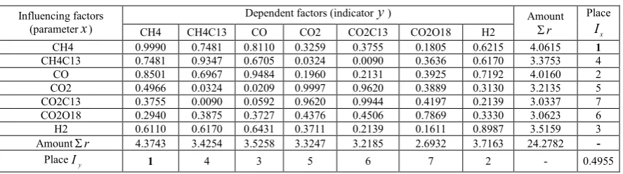
Table 9. Correlation matrix and rating of factors after the trend (1) of binary relations and two wavelets (4) dynamics

Influencing factors (parameterx)

Dependent factors (indicatory) _Amount

r



Place x

I

CH4 CH4C13 CO CO2 CO2C13 CO2O18 H2

CH4 0.9990 0.7481 0.8110 0.3259 0.3755 0.1805 0.6215 4.0615 1 CH4C13 0.7481 0.9347 0.6705 0.0324 0.0090 0.3636 0.6170 3.3753 4 CO 0.8501 0.6967 0.9484 0.1960 0.2131 0.3925 0.7192 4.0160 2 CO2 0.4966 0.0324 0.0209 0.9997 0.9620 0.3889 0.3130 3.2135 5 CO2C13 0.3755 0.0090 0.0592 0.9620 0.9944 0.4197 0.2139 3.0337 7 CO2O18 0.2940 0.3875 0.3727 0.4376 0.4506 0.7869 0.3330 3.0623 6 H2 0.6110 0.6170 0.6431 0.3711 0.2139 0.1611 0.8987 3.5159 3 Amountr 4.3743 3.4254 3.5258 3.3247 3.2185 2.6932 3.7163 24.2782 -

PlaceI_y 1 4 3 5 6 7 2 - 0.4955

[image:12.595.80.524.654.778.2]

The coefficient of correlation variation, that is, a measure of

the functional relationship between the system parameters at a weather station, is 22.6245 / 72 = 0.4617. As the influencing variable in the first place was CH4, in the second - CO and in the third place - CH4C13. As a dependent indicator, CH4 again came in first place, but CO2 came in second, and CH4C13 also came in third. For assessment, CH4 and CO2 are becoming the most important greenhouse gases.

Factor analysis by identifying the wave equation: For four members of the general model (4), containing two terms of the trend (1) and two more wave equations of dynamics, the correlation coefficients were placed in the diagonal cells of the correlation matrix (Table 9). The coefficient of correlation variation is 24.2782 / 72 = 0.4955. The rating of influencing and dependent factors in comparison with table 8 has not changed only for the first place. The influencing variable in the ranking was CH4, CO, H2, C14C13, CO2, CO2O18 and CO2C13. The rating among greenhouse gases as dependent indicators (evaluation criteria) begins with CH4, H2, CO.

Binary relationships between greenhouse gases

Patterns of binary relations: Binary relations are necessary for assessing the level of adequacy of mutual relations between

accepted factors (Table 10). Due to the quantum entanglement of relations between meteorological factors, wave equations cannot be obtained according to (4), therefore, only the trend model (1) was adopted for identification. Many binary relations were identified only at the level of linear equations, applied at the initial level of identification. The values of the correlation coefficient give quantum certainty, and the difference will characterize the quantum entanglement of the relations between the gases.

Influence CH4: The influence of this gas on the other six factors occurs according to the two-term formulas from the table 10 of the trend (Fig. 15). The greatest influence of CH4 has on the change in CO with a correlation coefficient of 0.8110. From the location of the points near the trend line, it is seen that no pattern is visible.In the graphs of the effect of CH4 on the change in CO and CO2C13, two clusters can be seen above and below the trend lines.

InfluenceCH4C13: This effect is shown by the graphs in Figure 16, which were constructed by the equations from Table 10. A comparison shows that this greenhouse gas has the greatest effect on CH4 with a correlation coefficient of 0.7481. Table 10. Parameters of the model (1) of binary relations between gases

Variable x Indicatory Тренд = (− ) + (− ) Correl.

coeffic.

r

Exponential law Biotechnical law

a _b c _d e _f g

CH4 CH4C13 -41.49063 0 0 -0.0031604 1 0 0 0.7481

CO -153.79890 -0.00083892 0.97705 3.17443e-7 2.85987 0 0 0.8110 CO2 -337.88549 1.15359e-7 0.33224 0.31829 1.15348 0.00051676 0.99984 0.3259

CO2C13 -5.05258 0 0 -0.0017340 1 0 0 0.3755

CO2O18 4.16594 0 0 -0.0017309 1 0 0 0.1805

H2 0.15168 -0.0044864 0.72021 -3.66043e-28 9.47767 0 0 0.6215

CH4C13 CH4 -6587.4737 0 0 -177.08830 1 0 0 0.7481

CO -5332.4994 0 0 -114.72851 1 0 0 0.6705

CO2 483.50566 0 0 2.43253 1 0 0 0.0324

CO2C13 -7.50663 0 0 0.0094812 1 0 0 0.0090

CO2O18 37.31397 0 0 0.76973 1 0 0 0.3636

H2 4838.7154 0 0 91.62938 1 0 0 0.6170

CO CH4 4363.5057 0.15026 0.60257 0.88119 1.85685 0.00048461 1.72830 0.8501 CH4C13 -48.21786 0.0020625 1.11044 -0.010916 1.68526 0.0027190 1.21687 0.6967

CO2 367.48788 -0.00012595 1 -1.14018e-47 25.72010 0 0 0.1960

CO2C13 -11.59263 0.0091071 1.24350 -0.0016549 2.22410 0.0050259 1.29569 0.2131

CO2O18 1.52726 -0.021079 1 -0.0074264 1.55257 0 0 0.3925

H2 264.38723 -0.18954 0.59018 -1.88183 1.65031 0 0 0.7192

CO2

CH4 -48703.945 -0.00047977 0.66607 20.19113 1.57617 0.0028770 1.05501 0.4966

CH4C13 -47.10521 0 0 0.00043185 1 0 0 0.0324

CO 22.61184 -0.0042306 1 -1.29648e-7 3.35935 0 0 0.0209

CO2C13 -3.15121 0 0 -0.013239 1 0 0 0.9620

CO2O18 -2.67735 -0.0012984 0.69678 0.0099731 1.01744 0 0 0.3889

H2 394.94980 -0.0031136 0.96241 -0.00025181 2.43712 0 0 0.3130

CO2C13 CH4 1071.47331 0 0 -81.33127 1 0 0 0.3755

CH4C13 -46.87688 0 0 0.0085604 1 0 0 0.0090

CO -21.87599 0 0 -9.33295 1 0 0 0.0592

CO2 -192.74099 0 0 -69.90462 1 0 0 0.9620

CO2O18 -5.94913 0 0 -0.88691 1 0 0 0.4197

H2 787.12277 0 0 31.16895 1 0 0 0.2139

CO2O18 CH4 1234.1114 -2.07572 0.20944 -8104.7096 0.53921 0 0 0.2940

CH4C13 -46.66626 -0.023879 0.99774 5.09121 3.63433 1.83740 1.00137 0.3875 CO 81.22510 0.30417 1 -1.77963 9.82059 0.00064084 33.0408 0.3727 CO2 360.23985 -0.019095 1.46535 1.40657e-141 1211.0084 0.070861 21.1785 0.4376

CO2C13 -7.88005 -0.016387 1 -1.24360e-6 33.57184 0 0 0.4506

H2 14.82953 0.0023404 24.07981 516.78494 0.11108 0 0 0.3330

H2 CH4 308.39428 -0.010137 0.91878 -1.49855e-7 3.89317 0 0 0.6110

CH4C13 -49.17754 0 0 0.0041555 1 0 0 0.6170

CO 0.015601 -0.018976 1.00472 -8.68505e-32 12.37004 0 0 0.6431 CO2 1974.0110 -0.0018342 1.01392 -1.17186 1.37470 0.00047731 0.96288 0.3711

CO2C13 -8.83248 0 0 0.0014679 1 0 0 0.2139

[image:14.595.89.512.48.416.2]

Fig. 15. Effect of CH4 on other greenhouse gases

Fig. 16. Effect of CH4C13 on other greenhouse gases

Influence CO: This gas affects the rest according to clearly nonlinear laws (Fig. 17).

[image:15.595.118.501.89.423.2]

The greatest influence of CO has on the greenhouse gas CH4 with a correlation coefficient of 0.8501.

Fig. 17. Effect of CO on other greenhouse gases

[image:15.595.123.492.444.769.2]

Influence CO2: The effect of this greenhouse gas on the other six species under Antarctica is shown in Figure 18. The greatest influence of CO2 is on CO2C13 with a correlation of 0.9620. The graph shows that with an increase in CO2, a decrease in CO2C13 occurs.

Influence CO2C13: Influence graphs are shown in Figure 19.

The greatest effect on CO2 occurs with a correlation coefficient of 0.9620. In this regard, these two greenhouse gases were mutually reversible.

[image:16.595.126.479.150.458.2]

Influence CO2O18: Figure 20 shows that the distribution of points near the trend line is more uniform. In Figure 19, it was seen that the dots form complex patterns.

Fig. 19. Effect of CO2C13 on other greenhouse gases

Fig. 20. Effect of CO2O18 on other greenhouse gases

[image:16.595.128.474.484.786.2]

With a weak factor bond of 0.4506, this greenhouse gas exerts CO2C13.

Influence H2: Similarly, with a uniform distribution of points near the trend line, H2 has an effect on other greenhouse gases (Fig. 21). This gas with a correlation coefficient of 0.6431 affects CO.

Conclusion

For each terrestrial weather station, it is necessary to study the point distributions of meteorological measurements. Many wavelets of meteorological parameters dynamics will make it possible to reveal quanta of climate and weather behavior for different time quanta: long-term, annual, plant ontogenesis period, seasonal, monthly, weekly, daily, hourly and minutely. These quanta of time measurement are divided into two parts: from many years to a month and from a week to a minute. For the first part of the dynamics data, it is possible to bring the wavelet identification process to the achievement of measurement error. The result is a high quantum certainty and low quantum entanglement. And for the second part, as a rule, due to the insufficient accuracy of the devices, the so-called noise appears and a high uncertainty of the wave patterns is obtained long before the measurement error.

Paired relationships provide insight into the quanta of interaction between factors. But they are identified only by trends, and of these, a significant part of binary relations is modeled only by a linear formula. The quantum entanglement of the dynamics and relations between meteorological parameters is calculated by the difference between 1 and the correlation coefficient of the revealed pattern. As a result, two types of behavior quanta are distinguished for greenhouse gases:

firstly, in dynamics, each factor is divided into the sum of

wavelets, that is, in time quanta the factor is represented as a bundle of solitary waves (solitons), and quantum certainty is achieved by identification;

secondly, the mutual influence of climatic and meteorological

factors with a uniform or uneven measurement scale additionally gets quantum entanglement at some boundaries of the dynamics of behavior.

[image:17.595.121.469.48.367.2]

Thus, any phenomenon or process is evaluated by the level of adequacy (correlation coefficient) of the decomposition of the functional connection of the behavior of the system of meteorological parameters in dynamics and the mutual Fig. 21. The effect of H2 on other greenhouse gases

Table 11. Comparison of the dynamics models of the greenhouse gases of Antarctica

Place Greenhouse gas

Oscillationcycle The form of an equation and the correlation

r

year

r

half a year

r

linear trend 4 members

r

_14

/

r

₀

1 CO2 5 0.8407 - - 0.9970 0.9994 0.9997 1.0027

2 CO2C13 7 0.7886 - - 0.9897 0.9919 0.9994 1.0098

3 CH4 4 0.9747 8 0.5626 0.9353 0.9776 0.9990 1.0681

4 CO 3* 0.9389 5 0.7114 0.1804 0.1827 0.9484 5.2572

5 CH4C13 4* 0.7715 8* 0.1353 0.7190 0.7860 0.9347 1.3000

6 H2 4 0.8569 7 0.3755 0.2425 0.3606 0.8987 3.7060

7 CO2O18 5 0.6427 - - 0.5972 0.6104 0.7869 1.3176

[image:17.595.74.517.407.514.2]

relations between members of the system into quantum certainty and quantum entanglement. As a rule, the first member of the model is a natural component, and the second in the trend and subsequent members of the model in the form of wavelets show biotechnical (according to V.I. Vernadsky), in particular, anthropogenic, influence. After identification by trend and two wave functions, the sequence of CH4, CO, H2, C14C13, CO2, CO2O18, and CO2C13 appeared in the ranking of influencing variables. The ranking among greenhouse gases as dependent indicators (evaluation criteria) begins with the triple of CH4, H2, CO. A comparison of the 4-membered equations for greenhouse gases is given in Table 11. Greenhouse gas CO2 has the highest linear correlation coefficient of 0.9970. A simple pattern was visible to everyone and therefore there are so many publications on CO2 gas. Its wavelet with a one-year cycle has a correlation coefficient of 0.8407, which was noted in (Graven et al., 2013). In Antarctica, due to the remoteness of the vegetation of South America and Australia, the semi-annual cycle is eroded and therefore little noticeable. However, it is present in other parts of the planet (Mazurkin, 2018). With the highest correlation coefficient 0.7114, CO is present in Antarctica, CH4 is in second place with 0.5626, and H2 is in third place with 0.3755. The main reason for the annual cycle is a change in the angle of inclination of the earth's axis. Even in Antarctica, according to table 11, the influence of this astronomical parameter on the fluctuation of greenhouse gases is noticeable. For any weather station and forests, the angle of incidence of sunlight is also important. And semi-annual cycles depend, as a rule, on the vegetation cover of both hemispheres. Apparently, the semiannual cycles of CH4 and CH4CO13 can be explained mainly by the presence of ammonia reserves in Antarctica. For seven greenhouse gases, the first member of the trend model is the law of Laplace (in mathematics), Mandelbrot (in physics), Zipf-Perl (in biology) and Pareto (in econometrics) that we modified. It shows exponential growth or decline over time.

REFERENCES

Folland, C.K., O. Boucher, A. Colman, D.E. Parker, 2018: Causes of irregularities in trends of global mean surface temperature since the late 19th century. Science advances,

4 (6). DOI: 10.1126/sciadv.aao5297.

Forkel, M., N. Carvalhais, C. Rödenbeck, et al., 2016: Enhanced seasonal CO2 exchange caused by amplified plant productivity in northern ecosystems. Science, 351, 6274, 606-700. DOI: 10.1126/science.aac4971.

Friedrich, T., A. Timmermann, M. Tigchelaar, O.E. Timm, A. Ganopolski, 2016: Nonlinear climate sensitivity and its implications for future greenhouse warming. SciAdv2 (11), e1501923. DOI: 10.1126/sciadv.1501923.

Graven, H.D., R.F. Keeling, S.C. Piper, et al., 2013: Enhanced Seasonal Exchange of CO2 by Northern Ecosystems Since 1960. Science express, 311, 6150, 1085-1089. DOI 10.1126/scince.1239207.

Mazurkin, P.M., 2014: Method of identification. International Multidisciplinary Scientific GeoConference, Geology and

Mining Ecology Management, SGEM, 1(6), 427-434.

https://www.scopus.com/inward/record.uri?eid=2-s2.0-84946541076&partnerID=40&md5=72a3fcce31b20f2e63 e4f23e9a8a40e3.

Mazurkin, P.M., 2018:Wave patterns of annual global carbon dynamics (according to information Global_Carbon_ Budget_2017v1.3.xlsx). Materials of the International

Conference “Research transfer”Reports in English (part

2). November 28. Beijing, PRC. P.164-191.

Mazurkin, P.M., and A.I. Kudrjashova, 2018: Factor analysis of annual global carbon dynamics (according to Global_Carbon_Budget_2017v1.3.xlsx). Materials of the

International Conference “Research transfer” Reports in

English (part 2). November 28. Beijing, PRC. P.192-224.

Meinshausen, M., S.J. Smith, K. Calvin, et al., 2011: The RCP greenhouse gas concentrations and their extensions from 1765 to 2300. Climatic Change. 2011. DOI 10.1007/s10584-011-0156-z.

Quéré, C.L, R.M. Andrew, P. Friedlingstein, et al., 2018: Global Carbon Budget 2019. Earth Syst. Sci. Data, 10, 2141–2194. https://doi.org/10.5194/essd-10-2141-2018. Sejas, S.A., P.C. Taylor, M. Cai, 2018: Unmasking the

negative greenhouse effect over the Antarctic Plateau.

Climate and Atmospheric Science, 1:17. doi:10.1038/

s41612-018-0031-y.

*******