Finite Time Bounded Tracking Control for Linear Discrete Time Systems

(1)

Liao, F and Wu, Y and Yu, X and Deng, J (2018) Finite-Time Bounded Tracking Control for Linear

Discrete-Time Systems.

Mathematical Problems in Engineering, 2018.

ISSN 1024-123X DOI:

https://doi.org/10.1155/2018/7017135

Link to Leeds Beckett Repository record:

http://eprints.leedsbeckett.ac.uk/5219/

Document Version:

Article

Creative Commons: Attribution 4.0

The aim of the Leeds Beckett Repository is to provide open access to our research, as required by

funder policies and permitted by publishers and copyright law.

The Leeds Beckett repository holds a wide range of publications, each of which has been

checked for copyright and the relevant embargo period has been applied by the Research Services

team.

We operate on a standard take-down policy.

If you are the author or publisher of an output

and you would like it removed from the repository, please

contact us

and we will investigate on a

case-by-case basis.

(2)

Research Article

Finite-Time Bounded Tracking Control for

Linear Discrete-Time Systems

Fucheng Liao

,

1,2

Yingxue Wu,

1,2

Xiao Yu,

1,2

and Jiamei Deng

3 1_{Department of Information and Computing Science, School of Mathematics and Physics,}

University of Science and Technology Beijing, Beijing 100083, China

2_{Beijing Key Laboratory for Magneto-Photoelectrical Composite and Interface Science, School of Mathematics and Physics,} University of Science and Technology Beijing, Beijing 100083, China

3_{School of Computing, Creative Technologies and Engineering, Leeds Beckett University, Leeds, LS6 3QS, UK} Correspondence should be addressed to Jiamei Deng; [email protected]

Received 20 November 2017; Revised 4 May 2018; Accepted 21 May 2018; Published 25 June 2018

Academic Editor: Franck J. Vernerey

Copyright © 2018 Fucheng Liao et al. This is an open access article distributed under the Creative Commons Attribution License, which permits unrestricted use, distribution, and reproduction in any medium, provided the original work is properly cited.

A finite-time bounded tracking control problem for a class of linear discrete-time systems subject to disturbances is investigated. Firstly, by applying a difference method to constructing the error system, the problem is transformed into a finite-time boundedness problem of the output vector of the error system. In fact, this is a finite-time boundedness problem with respect to the partial variables. Secondly, based on the partial stability theory and the research methods of finite-time boundedness problem, a state feedback controller formulated in form of linear matrix inequality is proposed. Based on this, a finite-time bounded tracking controller of the original system is obtained. Finally, a numerical example is presented to illustrate the effectiveness of the controller.

1. Introduction

In 1961, Dorato proposed the concept of finite-time stability (FTS) in [1]. The main concept is that if the bound of the initial condition is given, the state of the system does not exceed a certain bound over a given finite time-interval. Since then, many scholars have conducted indepth research on FTS. In the 1960s, Kushner investigated the FTS of stochastic systems in [2]. Weiss and Infante discussed the FTS of nonlinear systems in [3, 4]. However, due to the lack of effective math-ematical tools at that time, the research progress is relatively slow.

With the development of linear matrix inequality (LMI) theory, the research on FTS yielded fruitful results. In [5, 6], Amato et al. extended the concept of FTS to the linear con-tinuous-time system with external disturbances and pre-sented the concept of finite-time boundedness (FTB). The FTB of time-varying continuous-time systems was discussed in [7]. Subsequently, the discrete-time system was investi-gated in [8, 9] and further research was done in [10–12]. In

[10], the state feedback controller and output feedback con-troller were designed to guarantee the FTB of the discrete-time system with disturbance. In [11], the FTS of discrete sys-tems was analyzed by using polyhedral Lyapunov function. In [12], the sufficient conditions for FTS of time-varying discrete systems were given and an output feedback controller was developed.

Following the pioneering work of Amato et al., many

scholars extended the research of FTB of discrete-time sys-tems. In [13], the finite-time control for linear discrete-time system with external disturbances was studied. The FTS of discrete-time stochastic systems with time-varying delays and its application to multiagent systems were considered in [14]. In [15], a finite-time optimal control method for a class of linear discrete-time systems with parameter variation was presented. By constructing the Lyapunov-Krasovskii func-tional, the FTS of discrete time-delay systems with nonlinear perturbations was studied in [16]. In [17], a robust controller was proposed to address the finite-time control problem of linear uncertain discrete systems by using an augmented LMI

(3)

method. In [18], the FTS and𝐻_∞control problem of discrete-time systems were discussed and a robust finite-discrete-time control scheme was provided.

On the basis of [13], the tracking control problem of linear discrete-time systems with disturbances in a finite time-interval is considered in this paper. Firstly, the error system is constructed based on the preview control theory [19, 20], and the problem is turned into a FTB problem of the output vector of the error system. Then a state feedback controller is designed for the error system via the LMI approach. Finally, a finite-time state feedback controller of the original system is derived.

Throughout this paper, the following notations are

adopted. Matrix𝑃 > 0(or𝑃 < 0) means that𝑃is symmetric

positive definite (or negative definite).𝑃 ≥ 0(𝑃 ≤ 0) means

that𝑃is symmetric positive semidefinite (or negative

semi-definite).𝑃 > 𝑄(𝑃 < 𝑄,𝑃 ≥ 𝑄, and𝑃 ≤ 𝑄) means that

𝑃 − 𝑄 > 0(𝑃 − 𝑄 < 0,𝑃 − 𝑄 ≥ 0, and𝑃 − 𝑄 ≤ 0).𝜆_max(𝐴)

(𝜆min(𝐴)) denotes the maximal (or minimal) eigenvalue of a

real symmetric matrix𝐴. diag(. . .)denotes a block-diagonal

matrix.

2. Preliminaries and Basic Concepts

This paper considers the following linear discrete-time sys-tem:

𝑥 (𝑘 + 1) = 𝐴𝑥 (𝑘) + 𝐸𝑤 (𝑘) , (1)

where𝑥(𝑘) ∈ 𝑅𝑛and𝑤(𝑘) ∈ 𝑅𝑝are the state vector and the

disturbance vector of the system, respectively.𝐴 ∈ 𝑅𝑛×𝑛and

𝐸 ∈ 𝑅𝑛×𝑝_{are known constant matrices.}

In [10–13], the FTB problem of system (1) was investigated and its basic definition was described as follows: system (1) is

said to be finite-time bounded with respect to(𝛿, 𝑑, 𝜀, 𝑅, 𝑁),

where𝑁 ≥ 1,𝑑 > 0,𝜀 > 0,𝛿 > 0, and𝑅 > 0, if

𝑥𝑇(0) 𝑅𝑥 (0) ≤ 𝛿2,

𝑁

∑

𝑘=0

𝑤𝑇(𝑘) 𝑤 (𝑘) ≤ 𝑑2󳨐⇒

𝑥𝑇(𝑘) 𝑅𝑥 (𝑘) ≤ 𝜀2,

∀𝑘 ∈ {1, 2, ⋅ ⋅ ⋅ , 𝑁} .

(2)

For convenience, hereinafter, the state vector of system (1) is also said to be finite-time bounded with respect to

(𝛿, 𝑑, 𝜀, 𝑅, 𝑁). The object of this paper is to generalize this concept and further study the finite-time bounded tracking problem of control systems. In the following, we first propose a definition of finite-time bounded tracking. Consider the discrete-time system

𝑥 (𝑘 + 1) = 𝐴𝑥 (𝑘) + 𝐸𝑤 (𝑘) ,

𝑦 (𝑘) = 𝐶𝑥 (𝑘) , (3)

where𝑥(𝑘) ∈ 𝑅𝑛,𝑤(𝑘) ∈ 𝑅𝑝, 𝑦(𝑘) ∈ 𝑅𝑞,𝐴 ∈ 𝑅𝑛×𝑛, and

𝐸 ∈ 𝑅𝑛×𝑝.

In some practical problems, it is hoped that the output of

system (3) is always located in a𝜀neighborhood of a reference

signal under some certain conditions. This kind of problem is referred to as “finite-time bounded tracking problem.” Let

the reference signal be𝑟(𝑘) ∈ 𝑅𝑞. And the error signal𝑒(𝑘)is

defined as

𝑒 (𝑘) = 𝑦 (𝑘) − 𝑟 (𝑘) . (4)

The concept mentioned above can be described by the following definition.

Definition 1. System (3) achieves finite-time bounded

track-ing of the reference signal𝑟(𝑘)with respect to(𝛿, 𝑑, 𝜀, 𝑅, 𝑁),

where𝑁 ≥ 1,𝛿 > 0,𝑑 > 0,𝜀 > 0, and𝑅 > 0, if

𝑒𝑇(0)Re(0) ≤ 𝛿2,

𝑁

∑

𝑘=0

𝑤𝑇(𝑘) 𝑤 (𝑘) ≤ 𝑑2󳨐⇒

𝑒𝑇(𝑘)Re(𝑘) ≤ 𝜀2,

∀𝑘 ∈ {1, 2, ⋅ ⋅ ⋅ , 𝑁} .

(5)

Remark 2. The conclusion of Definition 1 is equivalent to the

fact that the error signal𝑒(𝑘) is finite-time bounded with

respect to(𝛿, 𝑑, 𝜀, 𝑅, 𝑁); that is, the output𝑦(𝑘)of system (3)

is always located in the𝜀neighborhood of the reference signal

𝑟(𝑘)within a given time-interval{1, 2, ⋅ ⋅ ⋅ , 𝑁}.

In [13], the sufficient conditions for FTB of system (1) with

respect to(𝛿, 𝑑, 𝜀, 𝑅, 𝑁)were presented in terms of LMI. In

this paper, the research methods in [13] will be modified and combined with the error system method in preview control theory to study the finite-time bounded tracking problem.

The Schur complement lemma is needed to deduce an LMI feasibility problem.

Lemma 3(see [21]). Symmetric matrix[𝑆_𝑆11𝑇 𝑆12

12𝑆22] < 0if and

only if one of the following two conditions is satisfied:

(1)𝑆₁₁< 0, 𝑆₂₂− 𝑆𝑇₁₂𝑆−1₁₁𝑆₁₂< 0.

(2)𝑆₂₂< 0, 𝑆₁₁− 𝑆₁₂𝑆−1₂₂𝑆𝑇₁₂< 0.

3. Problem Description

Let us consider the linear discrete-time system with distur-bance

𝑥 (𝑘 + 1) = 𝐴𝑥 (𝑘) + 𝐵𝑢 (𝑘) + 𝐸𝑤 (𝑘) ,

𝑦 (𝑘) = 𝐶𝑥 (𝑘) , (6)

where𝑥(𝑘) ∈ 𝑅𝑛,𝑢(𝑘) ∈ 𝑅𝑚,𝑤(𝑘) ∈ 𝑅𝑝, and𝑦(𝑘) ∈ 𝑅𝑞are the

state vector, the input vector, the disturbance vector, and the

output vector of the system, respectively.𝐴 ∈ 𝑅𝑛×𝑛,𝐵 ∈ 𝑅𝑛×𝑚,

𝐸 ∈ 𝑅𝑛×𝑝_{, and}_{𝐶 ∈ 𝑅}𝑞×𝑛_{are known constant matrices.}

The difference operatorΔis defined as

(4)

The reference signal is𝑟(𝑘) ∈ 𝑅𝑞, and the error signal is defined by (4). The assumptions on disturbance signal and reference signal of system (7) are presented as follows:

A1: Assume that the disturbance vector satisfies the

condition,∑𝑁_𝑗=1Δ𝑤𝑇(𝑗)Δ𝑤(𝑗) ≤ 𝑑2₁, where𝑑₁> 0.

A2:Assume that the reference signal satisfies the

condi-tion,∑𝑁_𝑗=1Δ𝑟𝑇(𝑗)Δ𝑟(𝑗) ≤ 𝑑2₂, where𝑑₂> 0.

The purpose of this paper is to design a controller with preview action for linear discrete-time system (6) so that the closed-loop system can achieve the finite-time bounded

tracking of the reference signal𝑟(𝑘)with respect to(𝛿, 𝑑, 𝜀, 𝑅,

𝑁).

To achieve the above objective, an error system that

includes the information of the error signal𝑒(𝑘)will be first

constructed. Then, the error signal is considered as the output vector of this system. By this means, the original problem is converted into a FTB problem of the output vector of the error system.

4. Derivation of the Error System

Taking the operatorΔon both sides of the first equation of

(6), it follows that

Δ𝑥 (𝑘 + 1) = 𝐴Δ𝑥 (𝑘) + 𝐵Δ𝑢 (𝑘) + 𝐸Δ𝑤 (𝑘) . (8)

ApplyingΔto𝑒(𝑘 + 1) = 𝑦(𝑘 + 1) − 𝑟(𝑘 + 1)and noting that

Δ𝑒(𝑘 + 1) = 𝑒(𝑘 + 1) − 𝑒(𝑘), the following is obtained:

𝑒 (𝑘 + 1) = 𝑒 (𝑘) + Δ𝑦 (𝑘 + 1) − Δ𝑟 (𝑘 + 1) = 𝑒 (𝑘) + 𝐶Δ𝑥 (𝑘 + 1) − Δ𝑟 (𝑘 + 1)

= 𝑒 (𝑘) + 𝐶𝐴Δ𝑥 (𝑘) + 𝐶𝐵Δ𝑢 (𝑘) + 𝐶𝐸Δ𝑤 (𝑘) − Δ𝑟 (𝑘 + 1) .

(9)

Introduce the formal state vector𝑋₀(𝑘) = [_Δ𝑥(𝑘)𝑒(𝑘) ]and

matri-cesΦ = [_{0 𝐴}𝐼 𝐶𝐴],𝐺 = [𝐶𝐵_𝐵 ],𝐺_𝑟 = [−𝐼₀], and𝐺_𝑤= [𝐶𝐸_𝐸]. Com-bining (8) and (9) yields

𝑋₀(𝑘 + 1) = Φ𝑋₀(𝑘) + 𝐺Δ𝑢 (𝑘) + 𝐺_𝑟Δ𝑟 (𝑘 + 1)

+ 𝐺_𝑤Δ𝑤 (𝑘) . (10)

Define the new output

𝑒 (𝑘) = 𝐶0𝑋0(𝑘) , (11)

where𝐶₀ = [𝐼 0]. Thus, we can obtain the following error

system:

𝑋₀(𝑘 + 1) = Φ𝑋₀(𝑘) + 𝐺Δ𝑢 (𝑘) + 𝐺_𝑟Δ𝑟 (𝑘 + 1) + 𝐺_𝑤Δ𝑤 (𝑘) ,

𝑒 (𝑘) = 𝐶0𝑋0(𝑘) .

(12)

Since 𝑦(𝑘) = 𝐶𝑥(𝑘) is the output equation of system

(6),𝑦(𝑘)is measurable. Moreover, the reference signal𝑟(𝑘)

is known in advance. Thus, it is reasonable to consider𝑒(𝑘)as

the output vector of system (10).

Based on the above discussion, the finite-time bounded tracking problem of system (6) is transformed into the FTB

problem of the output vector𝑒(𝑘)of the closed-loop system

of error system (12).

5. Design of the Controller

Let us consider the following state feedback controller:

Δ𝑢 (𝑘) = 𝐾𝑋0(𝑘) , (13)

where𝐾 = [𝐾_𝑒 𝐾_𝑥]will be determined later. Applying this

controller to system (12) results in

𝑋₀(𝑘 + 1) = (Φ + 𝐺𝐾) 𝑋₀(𝑘) + 𝐺_𝑟Δ𝑟 (𝑘 + 1) + 𝐺_𝑤Δ𝑤 (𝑘) ,

𝑒 (𝑘) = 𝐶0𝑋0(𝑘) .

(14)

Compared with system (3), it can be seen that system (14)

is exactly same as system (3) except𝐺_𝑟Δ𝑟(𝑘+1). Hence,Δ𝑟(𝑘+

1)can be treated as the external disturbance. Putting𝐺_𝑟Δ𝑟(𝑘+

1)and𝐺_𝑤Δ𝑤(𝑘)together, a new disturbance vector𝑊(𝑘) =

[ Δ𝑤(𝑘)

Δ𝑟(𝑘+1)]is obtained. In this way, the closed-loop system (14)

becomes

𝑋₀(𝑘 + 1) = (Φ + 𝐺𝐾) 𝑋0(𝑘) + 𝐸𝑊 (𝑘) ,

𝑒 (𝑘) = 𝐶0𝑋0(𝑘) ,

(15)

where𝐸 = [𝐺_𝑤 𝐺_𝑟].

Remark 4. System (15) is now fully in the form of system (3), which will facilitate the controller design. Since system (15)

contains disturbancesΔ𝑟(𝑘+1)andΔ𝑤(𝑘), the corresponding

assumptions can be relaxed to A1 and A2. For 𝑤(𝑘), it

is easy to prove that A1 is much weaker than that of

∑𝑁_𝑘=0𝑤𝑇(𝑘)𝑤(𝑘) ≤ 𝑑2₁. In fact, if∑𝑁_𝑘=0𝑤𝑇(𝑘)𝑤(𝑘) ≤ 𝑑2₁/4, then A1 is satisfied. This is because

𝑁

∑

𝑘=1

Δ𝑤𝑇(𝑘) Δ𝑤 (𝑘) =∑𝑁

𝑘=1

(𝑤 (𝑘) − 𝑤 (𝑘 − 1))𝑇(𝑤 (𝑘)

− 𝑤 (𝑘 − 1)) ≤∑𝑁

𝑘=1

(‖𝑤 (𝑘)‖ + ‖𝑤 (𝑘 − 1)‖)2

=∑𝑁

𝑘=1(‖𝑤 (𝑘)‖

2_{+ ‖𝑤 (𝑘 − 1)‖}2

+ 2 ‖𝑤 (𝑘)‖ ‖𝑤 (𝑘 − 1)‖) ≤∑𝑁

𝑘=1

(2 ‖𝑤 (𝑘)‖2

+ 2 ‖𝑤 (𝑘 − 1)‖2) =∑𝑁

𝑘=1

(2𝑤𝑇(𝑘) 𝑤 (𝑘)

(5)

+ 2𝑤𝑇(𝑁) 𝑤 (𝑁) + 4𝑁−1∑

𝑘=1

𝑤𝑇(𝑘) 𝑤 (𝑘) ≤ 4∑𝑁

𝑘=0

𝑤𝑇(𝑘)

⋅ 𝑤 (𝑘) ≤ 𝑑2₁.

(16)

So far, the original problem has been converted into a FTB

problem of partial variable𝑒(𝑘)of system (15). The conclusion

of [13] cannot be directly applied to system (15). Therefore, it is necessary to combine relative ideas on partial stability with the proof methods in [13] to obtain the results of this paper. The following Theorem 5 is the first main result of this paper.

Theorem 5. The closed-loop system (15) achieves finite-time bounded tracking of the reference signal𝑟(𝑘) with respect to

(𝛿, 𝑑, 𝜀, 𝑅, 𝑁), if for a given scalar𝛾 > 1, there exist matrices

𝑃1> 0,𝑃2> 0and scalars𝜆1> 0,𝜆2> 0such that

[ [

(Φ + 𝐺𝐾)𝑇_𝐶𝑇

0𝑃1𝐶0(Φ + 𝐺𝐾) − 𝛾𝐶𝑇0𝑃1𝐶0 (Φ + 𝐺𝐾)𝑇𝐶𝑇0𝑃1𝐶0𝐸

𝐸𝑇𝐶𝑇

0𝑃1𝐶0(Φ + 𝐺𝐾) 𝐸𝑇𝐶𝑇0𝑃1𝐶0𝐸 − 𝛾𝑃2

] ]

≤ 0, (17)

𝑅 < 𝑃₁< 𝜆₁𝑅, (18)

0 < 𝑃₂< 𝜆₂𝐼, (19)

𝜆₁𝛿2+ 𝜆₂𝑑2< 𝜀2

𝛾𝑁−1. (20)

Moreover, the controller isΔ𝑢(𝑘) = 𝐾𝑋₀(𝑘).

Proof. Construct the following Lyapunov function:

𝑉 (𝑒 (𝑘)) = 𝑒𝑇(𝑘) 𝑃₁𝑒 (𝑘) . (21)

Due to𝑃₁> 0,𝑉(𝑒)is a positive-definite quadratic form with

respect to𝑒. Then, with some mathematical operations, we

have

𝑉 (𝑒 (𝑘 + 1)) = 𝑒𝑇(𝑘 + 1) 𝑃₁𝑒 (𝑘 + 1) = (𝐶0𝑋0(𝑘 + 1))𝑇𝑃1(𝐶0𝑋0(𝑘 + 1))

= [𝐶₀(Φ + 𝐺𝐾) 𝑋₀(𝑘) + 𝐶₀𝐸𝑊 (𝑘)]𝑇𝑃₁[𝐶₀(Φ + 𝐺𝐾) 𝑋₀(𝑘) + 𝐶₀𝐸𝑊 (𝑘)]

= [𝑋𝑇

0(𝑘) 𝑊𝑇(𝑘)] [

[

(Φ + 𝐺𝐾)𝑇_𝐶𝑇 0

𝐸𝑇𝐶𝑇₀ ]_]𝑃1[𝐶0(Φ + 𝐺𝐾) 𝐶0𝐸] [ 𝑋₀(𝑘)

𝑊 (𝑘)]

= [𝑋𝑇

0(𝑘) 𝑊𝑇(𝑘)] [

[

(Φ + 𝐺𝐾)𝑇𝐶𝑇

0𝑃1𝐶0(Φ + 𝐺𝐾) (Φ + 𝐺𝐾)𝑇𝐶𝑇0𝑃1𝐶0𝐸

𝐸𝑇𝐶𝑇

0𝑃1𝐶0(Φ + 𝐺𝐾) 𝐸𝑇𝐶𝑇0𝑃1𝐶0𝐸

] ]

[𝑋0(𝑘) 𝑊 (𝑘)] .

(22)

If condition (17) holds, the following stands:

𝑉 (𝑒 (𝑘 + 1)) ≤ 𝛾𝑉 (𝑒 (𝑘)) + 𝛾𝑊𝑇_{(𝑘) 𝑃} 2𝑊 (𝑘)

≤ 𝛾𝑉 (𝑒 (𝑘))

+ 𝜆max(𝑃2) 𝛾𝑊𝑇(𝑘) 𝑊 (𝑘) .

(23)

Applying (23) iteratively leads to

𝑉 (𝑒 (𝑘)) ≤ 𝛾𝑉 (𝑒 (𝑘 − 1)) + 𝜆max(𝑃2) 𝛾𝑊𝑇(𝑘 − 1) ⋅ 𝑊 (𝑘 − 1) ≤ 𝛾 [𝛾𝑉 (𝑒 (𝑘 − 2))

+ 𝜆max(𝑃2) 𝛾𝑊𝑇(𝑘 − 2) 𝑊 (𝑘 − 2)] + 𝜆max(𝑃2)

⋅ 𝛾𝑊𝑇(𝑘 − 1) 𝑊 (𝑘 − 1) = 𝛾2𝑉 (𝑒 (𝑘 − 2))

+ 𝜆max(𝑃2) [𝛾2𝑊𝑇(𝑘 − 2) 𝑊 (𝑘 − 2)

+ 𝛾𝑊𝑇(𝑘 − 1) 𝑊 (𝑘 − 1)] ≤ ⋅ ⋅ ⋅ ≤ 𝛾𝑘−1𝑉 (𝑒 (1))

+ 𝜆max(𝑃2) 𝑘−1

∑

𝑗=1

𝛾𝑗𝑊𝑇(𝑘 − 𝑗) 𝑊 (𝑘 − 𝑗) .

(24)

Taking𝛾 > 1into account, it is easily obtained from (24) that

𝑉 (𝑒 (𝑘)) ≤ 𝛾𝑘−1[ [

𝑉 (𝑒 (1))

+ 𝜆max(𝑃2) 𝑘−1

∑

𝑗=1

𝑊𝑇(𝑘 − 𝑗) 𝑊 (𝑘 − 𝑗)] ] .

(6)

Thus for all𝑘 ∈ {1, 2, ⋅ ⋅ ⋅ , 𝑁}, we get

𝑉 (𝑒 (𝑘)) ≤ 𝛾𝑁−1[ [

𝑉 (𝑒 (1))

+ 𝜆max(𝑃2)

𝑁−1

∑

𝑗=1𝑊

𝑇_{(𝑁 − 𝑗) 𝑊 (𝑁 − 𝑗)]}

] .

(26)

By setting𝑑2= 𝑑2₁+ 𝑑2₂, the following is obtained:

𝑁−1

∑

𝑗=1

𝑊𝑇(𝑁 − 𝑗) 𝑊 (𝑁 − 𝑗)

=𝑁−1∑

𝑗=1

Δ𝑤𝑇(𝑁 − 𝑗) Δ𝑤 (𝑁 − 𝑗)

+𝑁−1∑

𝑗=1

Δ𝑟𝑇(𝑁 + 1 − 𝑗) Δ𝑟 (𝑁 + 1 − 𝑗)

=𝑁−1∑

𝑗=1

Δ𝑤𝑇(𝑗) Δ𝑤 (𝑗) +∑𝑁

𝑗=2

Δ𝑟𝑇(𝑗) Δ𝑟 (𝑗)

≤∑𝑁

𝑗=1

Δ𝑤𝑇_{(𝑗) Δ𝑤 (𝑗) +}_∑𝑁 𝑗=1

Δ𝑟𝑇_{(𝑗) Δ𝑟 (𝑗)}

≤ 𝑑2₁+ 𝑑2₂= 𝑑2.

(27)

Moreover,

𝑉 (𝑒 (1)) = [𝑅1/2𝑒 (1)]𝑇(𝑅−1/2𝑃₁𝑅−1/2) [𝑅1/2𝑒 (1)] . (28)

Denoting̃𝑃₁= 𝑅−1/2𝑃₁𝑅−1/2, it follows that

𝑉 (𝑒 (1)) ≤ 𝜆max(̃𝑃1) 𝑒𝑇(1)Re(1) . (29)

Substituting (27) and (29) into (26) yields the further estima-tion:

𝑉 (𝑒 (𝑘))

≤ 𝛾𝑁−1[𝜆max(̃𝑃1) 𝑒𝑇(1)Re(1) + 𝜆max(𝑃2) 𝑑2] .

(30)

Since condition (18) is equivalent to𝐼 < 𝑅−1/2𝑃₁𝑅−1/2< 𝜆₁𝐼,

i.e.,𝐼 < ̃𝑃₁< 𝜆₁𝐼, it can be obtained that

1 < 𝜆min(̃𝑃1) ≤ 𝜆max(̃𝑃1) < 𝜆1. (31)

In addition, condition (19) implies

0 < 𝜆min(𝑃2) ≤ 𝜆max(𝑃2) < 𝜆2. (32)

Hence, if (18) and (19) hold, it can be easily seen from (30) that

𝑉 (𝑒 (𝑘)) ≤ 𝛾𝑁−1(𝜆₁𝛿2+ 𝜆₂𝑑2) . (33)

On the other hand, because of𝜆_min(̃𝑃₁) > 1, then

𝑉 (𝑒 (𝑘)) = 𝑒𝑇(𝑘) 𝑃1𝑒 (𝑘) ≥ 𝜆min(̃𝑃1) 𝑒𝑇(𝑘)Re(𝑘)

≥ 𝑒𝑇(𝑘)Re(𝑘) .

(34)

According to (33) and (34), the following is obtained:

𝑒𝑇_(𝑘)_Re_{(𝑘) ≤ 𝛾}𝑁−1_(𝜆

1𝛿2+ 𝜆2𝑑2) . (35)

Condition (20) implies that𝛾𝑁−1(𝜆₁𝛿2+ 𝜆₂𝑑2) < 𝜀2. Then, it

can be concluded that𝑒𝑇(𝑘)Re(𝑘) ≤ 𝜀2(𝑘 ∈ {1, 2, ⋅ ⋅ ⋅ , 𝑁}).

This completes the proof.

By observing the inequality (17) carefully, it can be seen that (17) is not an LMI. Hence, it cannot be easily solved by Matlab LMI toolbox. To this end, a tractable LMI form will be presented in the following. This is the second main theorem of this paper.

Theorem 6. The closed-loop system (15) achieves finite-time bounded tracking of the reference signal𝑟(𝑘) with respect to

(𝛿, 𝑑, 𝜀, 𝑅, 𝑁), if for a given scalar𝛾 > 1, there exist matrices

𝑄₁> 0,𝑃₂> 0and scalars𝜆󸀠₁> 0,𝜆₂> 0such that

[ [ [ [ [ [ [

−𝛾𝑄1 0 0 (𝑄1+ 𝐶𝐵𝐿)𝑇

0 0 0 (𝐶𝐴 + 𝐶𝐵𝐾𝑥)𝑇

0 0 −𝛾𝑃2 ̃𝐸𝑇

(𝑄1+ 𝐶𝐵𝐿) (𝐶𝐴 + 𝐶𝐵𝐾𝑥) ̃𝐸 −𝑄1

] ] ] ] ] ] ] ≤ 0,

(36)

𝜆󸀠1𝑅−1< 𝑄1< 𝑅−1, (37)

0 < 𝑃2< 𝜆2𝐼, (38)

[ [

𝜆2𝑑2− 𝜀 2

𝛾𝑁−1 𝛿

𝛿 −𝜆󸀠1

] ]

< 0, (39)

where ̃𝐸 = [𝐶𝐸 −𝐼]. In this case the controller is Δ𝑢(𝑘) =

𝐾_𝑒𝑒(𝑘) + 𝐾_𝑥Δ𝑥(𝑘)with𝐾_𝑒= 𝐿𝑄−1₁ .

Proof. The key of the proof lies in that the conditions of Theorem 5 are satisfied if the condition of this theorem holds.

To convert (17) to an LMI, let𝑄₁ = 𝑃₁−1; then (17) can be

equivalently written as

[ [

(Φ + 𝐺𝐾)𝑇𝐶𝑇

0𝑄−11 𝐶0(Φ + 𝐺𝐾) − 𝛾𝐶0𝑇𝑄−11 𝐶0 (Φ + 𝐺𝐾)𝑇𝐶𝑇0𝑄−11 𝐶0𝐸

𝐸𝑇𝐶𝑇

0𝑄−11 𝐶0(Φ + 𝐺𝐾) 𝐸𝑇𝐶𝑇0𝑄−11 𝐶0𝐸 − 𝛾𝑃2

] ]

(7)

Since the equivalent transformation of this inequality cannot

yield the desired result, the matrix𝐾 = [𝐾_𝑒 𝐾_𝑥]and the

expressions of 𝐶₀, Φ, 𝐺, 𝐾, 𝐸, 𝐺_𝑟, and 𝐺_𝑤 in the

closed-loop system (15) are substituted into this inequality. Then the following can be obtained:

[ [ [ [ [ [

[𝐼 + 𝐶𝐵𝐾𝑒 𝐶𝐴 + 𝐶𝐵𝐾𝑥

𝐵𝐾𝑒 𝐴 + 𝐵𝐾𝑥

]

𝑇

[𝑄

−1

1 0

0 0] [

𝐼 + 𝐶𝐵𝐾𝑒 𝐶𝐴 + 𝐶𝐵𝐾𝑥

] − 𝛾 [𝑄

−1

1 0

0 0] [

]

𝑇

[𝑄

−1

1 0

0 0] [

𝐶𝐸 −𝐼

𝐸 0]

[𝐶𝐸 −𝐼

𝐸 0]

𝑇

[𝑄

−1

1 0

0 0] [

𝐵𝐾𝑒 𝐴 + 𝐵𝐾𝑥 ] [

𝐶𝐸 −𝐼

𝐸 0]

𝑇

[𝑄

−1

1 0

0 0] [

𝐶𝐸 −𝐼

𝐸 0] − 𝛾𝑃2

] ] ] ] ] ] ≤ 0, (41) that is, [ [ [ [ [ [ [

(𝐼 + 𝐶𝐵𝐾𝑒)𝑇𝑄−11 (𝐼 + 𝐶𝐵𝐾𝑒) − 𝛾𝑄−11 (𝐼 + 𝐶𝐵𝐾𝑒)𝑇𝑄1−1(𝐶𝐴 + 𝐶𝐵𝐾𝑥) (𝐼 + 𝐶𝐵𝐾𝑒)𝑇𝑄−11 𝐶𝐸 − (𝐼 + 𝐶𝐵𝐾𝑒)𝑇𝑄−11 (𝐶𝐴 + 𝐶𝐵𝐾_𝑥)𝑇𝑄−1

1 (𝐼 + 𝐶𝐵𝐾𝑒) (𝐶𝐴 + 𝐶𝐵𝐾𝑥)𝑇𝑄−11 (𝐶𝐴 + 𝐶𝐵𝐾𝑥) (𝐶𝐴 + 𝐶𝐵𝐾𝑥)𝑇𝑄−11 𝐶𝐸 − (𝐶𝐴 + 𝐶𝐵𝐾𝑥)𝑇𝑄−11 (𝐶𝐸)𝑇_𝑄−1

1 (𝐼 + 𝐶𝐵𝐾𝑒) −𝑄−1

1 (𝐼 + 𝐶𝐵𝐾𝑒)

(𝐶𝐸)𝑇_𝑄−1

1 (𝐶𝐴 + 𝐶𝐵𝐾𝑥) −𝑄−1

1 (𝐶𝐴 + 𝐶𝐵𝐾𝑥)

[(𝐶𝐸)

𝑇_𝑄−1

1 (𝐶𝐸) − (𝐶𝐸)𝑇𝑄−11 −𝑄−1

1 𝐶𝐸 𝑄−11

] − 𝛾𝑃₂ ] ] ] ] ] ] ] ≤ 0. (42)

Rewriting the left side of (42) yields

[ [ [ [ [ [ [

(𝐼 + 𝐶𝐵𝐾_𝑒)𝑇𝑄−1

1 (𝐼 + 𝐶𝐵𝐾𝑒) − 𝛾𝑄−11 (𝐼 + 𝐶𝐵𝐾𝑒)𝑇𝑄1−1(𝐶𝐴 + 𝐶𝐵𝐾𝑥) (𝐼 + 𝐶𝐵𝐾𝑒)𝑇𝑄−11 [𝐶𝐸 −𝐼]

(𝐶𝐴 + 𝐶𝐵𝐾_𝑥)𝑇𝑄−1

1 (𝐼 + 𝐶𝐵𝐾𝑒) (𝐶𝐴 + 𝐶𝐵𝐾𝑥)𝑇𝑄1−1(𝐶𝐴 + 𝐶𝐵𝐾𝑥) (𝐶𝐴 + 𝐶𝐵𝐾𝑥)𝑇𝑄−11 [𝐶𝐸 −𝐼]

[(𝐶𝐸)𝑇 −𝐼 ] 𝑄

−1

1 (𝐼 + 𝐶𝐵𝐾𝑒) [(𝐶𝐸)

𝑇

−𝐼 ] 𝑄

−1

1 (𝐶𝐴 + 𝐶𝐵𝐾𝑥) [(𝐶𝐸) 𝑇

−𝐼 ] 𝑄

−1

1 [𝐶𝐸 −𝐼] − 𝛾𝑃2

] ] ] ] ] ] ]

≤ 0. (43)

By denoting ̃𝐸 = [𝐶𝐸 −𝐼], the above inequality becomes

[ [ [ [

(𝐼 + 𝐶𝐵𝐾𝑒)𝑇𝑄−11 (𝐼 + 𝐶𝐵𝐾𝑒) − 𝛾𝑄−11 (𝐼 + 𝐶𝐵𝐾𝑒)𝑇𝑄1−1(𝐶𝐴 + 𝐶𝐵𝐾𝑥) (𝐼 + 𝐶𝐵𝐾𝑒)𝑇𝑄−11 ̃𝐸

(𝐶𝐴 + 𝐶𝐵𝐾𝑥)𝑇𝑄−11 (𝐼 + 𝐶𝐵𝐾𝑒) (𝐶𝐴 + 𝐶𝐵𝐾𝑥)𝑇𝑄−11 (𝐶𝐴 + 𝐶𝐵𝐾𝑥) (𝐶𝐴 + 𝐶𝐵𝐾𝑥)𝑇𝑄−11 ̃𝐸

̃𝐸𝑇_𝑄−1

1 (𝐼 + 𝐶𝐵𝐾𝑒) ̃𝐸𝑇𝑄−11 (𝐶𝐴 + 𝐶𝐵𝐾𝑥) ̃𝐸𝑇𝑄1−1̃𝐸 − 𝛾𝑃2

] ] ] ]

≤ 0. (44)

Pre- and postmultiplying (44) by the symmetric matrix diag(𝑄₁, 𝐼, 𝐼)and its transpose, respectively, we obtain

[ [ [ [

𝑄₁(𝐼 + 𝐶𝐵𝐾_𝑒)𝑇𝑄−1

1 (𝐼 + 𝐶𝐵𝐾𝑒) 𝑄1− 𝛾𝑄1 𝑄1(𝐼 + 𝐶𝐵𝐾𝑒)𝑇𝑄−11 (𝐶𝐴 + 𝐶𝐵𝐾𝑥) 𝑄1(𝐼 + 𝐶𝐵𝐾𝑒)𝑇𝑄−11 ̃𝐸

(𝐶𝐴 + 𝐶𝐵𝐾_𝑥)𝑇𝑄−1

1 (𝐼 + 𝐶𝐵𝐾𝑒) 𝑄1 (𝐶𝐴 + 𝐶𝐵𝐾𝑥)𝑇𝑄1−1(𝐶𝐴 + 𝐶𝐵𝐾𝑥) (𝐶𝐴 + 𝐶𝐵𝐾𝑥)𝑇𝑄−11 ̃𝐸

̃𝐸𝑇_𝑄−1

1 (𝐼 + 𝐶𝐵𝐾𝑒) 𝑄1 ̃𝐸𝑇𝑄−11 (𝐶𝐴 + 𝐶𝐵𝐾𝑥) ̃𝐸𝑇𝑄−11 ̃𝐸 − 𝛾𝑃2

] ] ] ]

(8)

In fact, (45) can be rewritten as

[ [ [

−𝛾𝑄₁ 0 0

0 0 0

0 0 −𝛾𝑃₂

] ] ]

−[[_[ [

𝑄1(𝐼 + 𝐶𝐵𝐾𝑒)𝑇

(𝐶𝐴 + 𝐶𝐵𝐾𝑥)𝑇

̃𝐸𝑇

] ] ] ]

(−𝑄₁)−1

⋅ [(𝐼 + 𝐶𝐵𝐾𝑒) 𝑄1 (𝐶𝐴 + 𝐶𝐵𝐾𝑥) ̃𝐸] ≤ 0.

(46)

From−𝑄₁< 0and Lemma 3 (2), (45) is equivalent to

[ [ [ [ [ [ [

−𝛾𝑄₁ 0 0 𝑄₁(𝐼 + 𝐶𝐵𝐾_𝑒)𝑇

0 0 0 (𝐶𝐴 + 𝐶𝐵𝐾𝑥)𝑇

0 0 −𝛾𝑃2 ̃𝐸𝑇

(𝐼 + 𝐶𝐵𝐾_𝑒) 𝑄₁ (𝐶𝐴 + 𝐶𝐵𝐾_𝑥) ̃𝐸 −𝑄₁

] ] ] ] ] ] ] ≤ 0.

(47)

By setting𝐿 = 𝐾_𝑒𝑄₁, it can be seen that (47) becomes (36)

and (17) is finally converted to an equivalent LMI (36).

Because of𝑄₁= 𝑃₁−1, (18) becomes

𝑅 < 𝑄−1₁ < 𝜆₁𝑅. (48)

Then the above equation leads to

1

𝜆₁𝑅−1< 𝑄1< 𝑅−1, (49)

which implies that 𝑄₁ needs to meet the condition:

(1/𝜆₁)𝑅−1− 𝑄₁< 0. Since𝜆₁ > 0and𝑄₁ > 0are unknown, this inequality cannot be solved by the LMI toolbox in Matlab.

Thus, let𝜆󸀠₁ = 1/𝜆₁; then (49) is converted into a

computa-tionally tractable condition (37).

Taking𝜆󸀠₁= 1/𝜆₁into account, (20) can be written as

1 𝜆󸀠

1𝛿

2_{+ 𝜆}

2𝑑2< 𝜀

2

𝛾𝑁−1. (50)

It is also necessary to convert (50) to an LMI. For this purpose, we rewrite (50) as

(𝜆₂𝑑2₋ 𝜀2

𝛾𝑁−1) − 𝛿 (−𝜆󸀠1) −1

𝛿 < 0. (51)

Because of −𝜆󸀠₁ < 0, it can be obtained by Lemma 3 (2)

that conditions (50) and (39) are equivalent. Besides, (19) in Theorem 5 does not require any change and it is (38). This completes the proof.

Note thatΔ𝑢(𝑘) = 𝑢(𝑘) − 𝑢(𝑘 − 1). By solving𝑢(𝑘), the

following result is derived instantly.

Theorem 7. Assume that A1-A2 are satisfied. The control input of linear discrete-time system (6) is given by

𝑢 (𝑘) = 𝑢 (0) + 𝐾𝑒 𝑘

∑

𝑗=1

𝑒 (𝑗) + 𝐾_𝑥(𝑥 (𝑘) − 𝑥 (0)) ,

𝑘 ∈ {1, 2, ⋅ ⋅ ⋅ , 𝑁} ,

(52)

where𝐾_𝑒and𝐾_𝑥are determined by LMIs (36)-(39). Under the controller, system (6) achieves finite-time bounded tracking of the reference signal𝑟(𝑘)with respect to(𝛿, 𝑑, 𝜀, 𝑅, 𝑁).

Remark 8. The results in this paper can be readily extended to linear discrete-time systems with state delay. In this case, we can construct a delay-free error system by applying the differ-ence method and the discrete lifting technique [22]. Further-more, the error vector is still taken as the output vector of the error system. Then, applying the controller design method in this paper, a finite-time bounded tracking controller of dis-crete time-delay systems can be obtained.

6. Simulation Example

The effectiveness of the proposed method will be shown by a numerical example, in which two different reference signals are considered.

Example 1. Consider system (6) with the following system matrices:

𝐴 = [1 2

−1 −2] ,

𝐵 = [−0.5 1 ] ,

𝐸 = [−0.1 0.5] , 𝐶 = [0.1 0.3] .

(53)

Take𝑅 = 𝐼,𝛿 = 0.1,𝑑 = √6/2,𝜀 = √5,𝑁 = 100, and

𝛾 = 1.01. By using the LMI toolbox in Matlab to solve the LMIs (36)-(39) in Theorem 6, the feedback gain matrices are given by

𝐾_𝑒 = −4,

𝐾_𝑥= [0.8 1.6] . (54)

Then let𝑥(0) = [0₀]and𝑢(0) = 0; we obtain

𝑢 (𝑘) = 𝑢 (0) + 𝐾𝑒 𝑘

∑

𝑗=1

𝑒 (𝑗) + 𝐾_𝑥(𝑥 (𝑘) − 𝑥 (0))

= −4∑𝑘

𝑗=1

𝑒 (𝑗) + 0.8𝑥₁(𝑘) + 1.6𝑥2(𝑘) .

(55)

The disturbance is taken as

𝑤 (𝑘) = 3sin0.07𝜋𝑘

(0.5 + 𝑘)0.6 . (56)

By calculation, we have

𝑁

∑

𝑗=1

(9)

Below, two different reference signals are considered to do the numerical simulation.

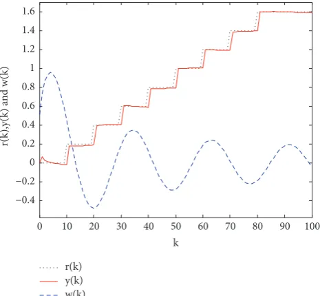
(1) The reference signal is taken as

𝑟 (𝑘) = { { { { { { { { { { { { { { { { { { { { { { { { { { { { { { { { { { { { { { { { { { { { { { {

0, 0 ≤ 𝑘 < 10, 0.2, 10 ≤ 𝑘 < 20, 0.4, 20 ≤ 𝑘 < 30, 0.6, 30 ≤ 𝑘 < 40, 0.8, 40 ≤ 𝑘 < 50, 1, 50 ≤ 𝑘 < 60, 1.2, 60 ≤ 𝑘 < 70, 1.4, 70 ≤ 𝑘 < 80, 1.6, 80 ≤ 𝑘 ≤ 100.

(58)

In this case,𝑟(𝑘)satisfies∑𝑁_𝑗=1Δ𝑟𝑇(𝑗)Δ𝑟(𝑗) = 0.32 ≤ 1def= 𝑑2₂.

Note that

𝑑2₁+ 𝑑2₂= 3

2 = 𝑑2. (59)

In addition, from𝑥(0) = [0₀]and𝑢(0) = 0,𝑒𝑇(1)Re(1) =

𝑒𝑇(1)𝑒(1) ≈ 0.0052can be obtained. Then the following con-dition is guaranteed:

𝑒𝑇₍₁₎_Re_{(1) ≤ 0.01 = 𝛿}2_. ₍₆₀₎ Therefore, the tracking error between the closed-loop output and the reference signal (58) should satisfy

𝑒𝑇(𝑘)Re(𝑘) ≤ 𝜀2 (𝑘 ∈ {1, 2, ⋅ ⋅ ⋅ , 100}) . (61) Figure 1 shows the output response of the closed-loop system, and Figure 2 shows the tracking error between the closed-loop output and the reference signal.

As shown in Figures 1-2, the proposed controller guar-antees that the closed-loop output signal is always in the

𝜀neighborhood of the reference signal𝑟(𝑘)within a given

time-interval{1, 2, ⋅ ⋅ ⋅ , 100} and the error signal is always

in a given range. That is to say, the closed-loop system achieves finite-time bounded tracking of the reference signal

𝑟(𝑘) with respect to (0.1, √6/2, √5, 𝐼, 100). It needs to be

emphasized that the tracking error is very small even if a strong disturbance signal exists in the system.

Note that from Definition 1, if𝑒𝑇(0)Re(0) ≤ 𝛿2and other

conditions are satisfied,𝑒𝑇(𝑘)Re(𝑘) ≤ 𝜀2 holds. This result

has nothing to do with the selection of initial state𝑥(0). But

in fact, due to𝑒(0) = 𝑦(0)−𝑟(0) = 𝐶𝑥(0)−𝑟(0), the initial state

𝑥(0)is still limited. In this example, If we let𝑥(0) = [−0.00083_−0.07 ]

and𝑢(0) = 0, this results in𝑒𝑇(1)Re(1) = 𝑒𝑇(1)𝑒(1) = 0.01 =

𝛿2_._{𝛾 = 1.01}_{is still taken to solve the corresponding LMIs.} In this case, the simulation results are completely consistent with the theoretical results, and they are omitted here.

Note that the reference signal (58) is very valuable in practice. In fact, the desired trajectory of a biped robot in the upslope process is usually in the form of function (58) [23].

r(k) y(k) −0.4 −0.2 0 0.2 0.4 0.6 0.8 1 1.2 1.4 1.6 r(k),y(k) a n d w(k)

10 20 30 40 50 60 70 80 90 100

0

k

[image:9.600.312.545.72.287.2]

w(k)

Figure 1: The output response of the closed-loop system to reference signal (58). −0.3 −0.25 −0.2 −0.15 −0.1 −0.05 0 0.05 0.1 0.15 trac kin g err o r

10 20 30 40 50 60 70 80 90 100

0

[image:9.600.310.545.333.514.2]

k

Figure 2: The tracking error of the closed-loop system to reference signal (58).

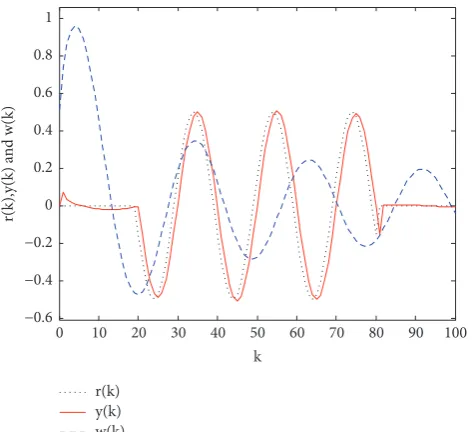
(2) The reference signal is taken as the periodic function given by

𝑟 (𝑘) = { { { { { { { { {

0, 80 < 𝑘 ≤ 100,

0.5sin[ 𝜋

10 (𝑘 − 10)] , 20 ≤ 𝑘 ≤ 80,

0, 0 ≤ 𝑘 < 20.

(62)

In this case, the following can be obtained:

𝑁

∑

𝑗=1

Δ𝑟𝑇(𝑗) Δ𝑟 (𝑗) ≈ 0.7819 ≤ 1def= 𝑑₂2, (63)

which implies∑𝑁_𝑗=1Δ𝑤𝑇(𝑗)Δ𝑤(𝑗) + ∑𝑁_𝑗=1Δ𝑟𝑇(𝑗)Δ𝑟(𝑗) ≤ 𝑑2.

(10)

r(k) y(k) w(k)

10 20 30 40 50 60 70 80 90 100

0

k −0.6

−0.4 −0.2 0 0.2 0.4 0.6 0.8 1

r(k),y(k) a

n

[image:10.600.53.290.71.287.2]

d w(k)

Figure 3: The output response of the closed-loop system to reference signal (62).

80 70

60 90 100

40 30 20

10 50

0

k −0.25

−0.2 −0.15 −0.1 −0.05 0 0.05 0.1 0.15 0.2 0.25

trac

kin

g err

o

[image:10.600.53.290.341.517.2]

r

Figure 4: The tracking error of the closed-loop system to reference signal (62).

Figure 3 shows the output response of the closed-loop system, and Figure 4 shows the tracking error between the actual output and the desired output. It can be seen that the closed-loop system achieves finite-time bounded tracking

of the reference signal𝑟(𝑘) with respect to(0.1, √6/2, √5,

𝐼, 100).

7. Conclusion

In this paper, the concept of finite-time bounded tracking control for linear discrete-time systems is proposed. Using the difference method, we construct an error system where the tracking error is only a part of the augmented state vector. Then, by constructing a Lyapunov function with respect to

the tracking error, a sufficient condition guaranteeing that the norm of tracking error is finite-time bounded is presented in terms of a set of LMIs. Based on this criterion, a feedback controller of the original system is derived, under which the closed-loop output achieves finite-time bounded tracking of the reference signal. Numerical simulation shows the effec-tiveness of the proposed controller.

Conflicts of Interest

No potential conflicts of interest was reported by the authors.

Funding

This work was supported by National Key R&D Program of China (no. 2017YFF0207401) and the Oriented Award Foundation for Science and Technological Innovation, Inner Mongolia Autonomous Region, China (no. 2012).

References

[1] P. Dorato, “Short time stability in linear time-varying systems,” inProceedings of the IRE international Convention Record Part 4, pp. 83–87, New York, NY, USA, May 1961.

[2] H. J. Kushner, “Finite time stochastic stability and the analysis of tracking systems,”IEEE Transactions on Automatic Control, vol. 11, no. 2, pp. 219–227, 1966.

[3] L. Weiss and E. F. Infante, “On the stability of systems defined over a finite time interval,”Proceedings of the National Acadamy of Sciences of the United States of America, vol. 54, pp. 44–48, 1965.

[4] L. Weiss and E. F. Infante, “Finite time stability under perturbing forces and on product spaces,”IEEE Transactions on Automatic Control, vol. AC-12, no. 1, pp. 54–59, 1967.

[5] F. Amato, M. Ariola, C. T. Abdallah, and P. Dorato, “Dynamic output feedback finite-time control of LTI systems subject to parametric uncertainties and disturbances,” inProceedings of the European Control Conference, pp. 1176–1180, Kalsruhe, Germany, September 1999.

[6] F. Amato, M. Ariola, C. T. Abdallah, and P. Dorato, “Finite-time control for uncertain linear systems with disturbance inputs,” in Proceedings of the American Control Conference, pp. 1776–1780, Calif, USA, June 1999.

[7] F. Amato, M. Ariola, and P. Dorato, “Finite-time control of linear systems subject to parametric uncertainties and distur-bances,”Automatica, vol. 37, no. 9, pp. 1459–1463, 2001. [8] F. Amato, M. Carbone, M. Ariola, and C. Cosentino,

“Finite-time stability of discrete-“Finite-time systems,” inProceedings of the 2004 American Control Conference (AAC), pp. 1440–1444, July 2004.

[9] F. Amato, M. Carbone, M. Ariola, and C. Cosentino, “Control of linear discrete-time systems over a finite-time interval,” in Pro-ceedings of the 43rd IEEE Conference on Decision and Control, pp. 1284–1288, Paradise island, Bahamas, January 2004. [10] F. Amato and M. Ariola, “Finite-time control of discrete-time

linear systems,”IEEE Transactions on Automatic Control, vol. 50, no. 5, pp. 724–729, 2005.

(11)

Control Conference, pp. 1656–1660, Washington, USA, June 2008.

[12] F. Amato, M. Ariola, and C. Cosentino, “Finite-time control of discrete-time linear systems: analysis and design conditions,” Automatica, vol. 46, no. 5, pp. 919–924, 2010.

[13] Y. J. Shen, “Finite-time control for a class of linear discrete-time systems,”Kongzhi yu Juece/Control and Decision, vol. 23, no. 1, pp. 107–109, 2008.

[14] M. Hu, J. Cao, A. Hu, Y. Yang, and Y. Jin, “A novel finite-time stability criterion for linear discrete-time stochastic system with applications to consensus of multi-agent system,”Circuits, Sys-tems and Signal Processing, vol. 34, no. 1, pp. 41–59, 2015. [15] K. Fujimoto, T. Inoue, and S. Maruyama, “On finite time

opti-mal control for discrete-time linear systems with parameter variation,” in Proceedings of the 54th IEEE Conference on Decision and Control, CDC 2015, pp. 6524–6529, December 2015.

[16] W. Kang, S. Zhong, K. Shi, and J. Cheng, “Finite-time stability for discrete-time system with time-varying delay and nonlinear perturbations,”ISA Transactions, vol. 60, pp. 67–73, 2016. [17] D. Rotondo, F. Nejjari, and V. Puig, “Dilated LMI

characteriza-tion for the robust finite time control of discrete-time uncertain linear systems,”Automatica, vol. 63, pp. 16–20, 2016.

[18] L. A. Tuan and V. N. Phat, “Finite-time stability and𝐻_∞ con-trol of linear discrete-time delay systems with norm-bounded disturbances,”Acta Mathematica Vietnamica, vol. 41, no. 3, pp. 481–493, 2016.

[19] F.-C. Liao, X.-J. Su, and Y.-L. Liao, “𝐻_∞guaranteed performance preview control for uncertain discrete systems with time-delay,” Gongcheng Kexue Xuebao/Chinese Journal of Engineering, vol. 38, no. 7, pp. 1008–1016, 2016.

[20] Y. Lu, F. Liao, J. Deng, and H. Liu, “Cooperative global opti-mal preview tracking control of linear multi-agent systems: an internal model approach,” International Journal of Systems Science, vol. 48, no. 12, pp. 2451–2462, 2017.

[21] L. Yu,Robust Control: Linear Matrix Inequality Method, Tsing-hua University Press, Beijing, China, 2002.

[22] F. Liao and Y. Guo, “Optimal preview control for discrete-time sys-tems in multirate output sampling,”Mathematical Problems in Engineering, vol. 2016, 10 pages, 2016.

(12)

Hindawi

www.hindawi.com Volume 2018

Mathematics

Journal of

Hindawi

Mathematical Problems in Engineering Applied Mathematics Hindawi

Probability and Statistics Hindawi

Hindawi

Mathematical PhysicsAdvances in

Complex Analysis

Journal of

Hindawi

Optimization

Journal of

Hindawi

www.hindawi.com Volume 2018 Engineering Mathematics

International Journal of

Hindawi

Operations Research

Journal of

Hindawi

Function Spaces

Abstract and Applied Analysis

Hindawi

International Journal of Mathematics and Mathematical Sciences

Hindawi

Hindawi Publishing Corporation

http://www.hindawi.com Volume 2013

Hindawi www.hindawi.com

World Journal

Volume 2018

Hindawi

www.hindawi.com Volume 2018Volume 2018

Numerical Analysis

Advances inAdvances in Discrete Dynamics in Nature and Society Hindawi

Hindawi www.hindawi.com

Differential Equations International Journal of

Volume 2018

Hindawi

Decision Sciences

Hindawi

Analysis

Hindawi

Stochastic Analysis

Submit your manuscripts at

http://eprints.leedsbeckett.ac.uk/5219/

Liao

Deng

https://doi.org/10.1155/2018/7017135

Hindawiwww.hindawi.com

Applied MathematicsJournal of

Probability and StatisticsHindawi

Complex AnalysisJournal of

OptimizationJournal of

Journal ofHindawi

Abstract and Applied Analysis

Hindawi Publishing Corporation http://www.hindawi.com

Discrete Dynamics in Nature and Society

Submit your manuscripts atwww.hindawi.com