International Journal of Mathematics and Mathematical Sciences Volume 2008, Article ID 283846,16pages
doi:10.1155/2008/283846
Research Article
The Weighted Fermat Triangle Problem
Yujin Shen and Juan Tolosa
Natural Sciences and Mathematics, The Richard Stockton College of New Jersey, Pomona, NJ 08240, USA
Correspondence should be addressed to Juan Tolosa,[email protected]
Received 29 June 2007; Accepted 13 September 2007
Recommended by Marco Squassina
We completely solve the generalized Fermat problem: given a triangleP1,P2,P3and three positive numbersλ1,λ2,λ3, find a pointPfor which the sumλ1P1Pλ2P2Pλ3P3Pis minimal. We show that the point always exists and is unique, and indicate necessary and sufficient conditions for the point to lie inside the triangle. We provide geometric interpretations of the conditions and briefly indicate a connection with dynamical systems.
Copyrightq2008 Y. Shen and J. Tolosa. This is an open access article distributed under the Creative Commons Attribution License, which permits unrestricted use, distribution, and reproduction in any medium, provided the original work is properly cited.
1. Introduction
Pierre Fermat1601–1665formulated the following problem.
Given a triangleABC, find a pointPsuch that the sum of the three distances fromPto the verticesA,B,Cis minimal.
In the literature, one can find various beautiful ways to solve the problem see, e.g., 1–4. In short, the answer is as follows. If every angle ofABCmeasures less than 120◦, then the pointPin the interior of the triangle such that∠AP B∠BP C∠CP A 120◦minimizes the sum of the three distances. If one of the angles ofABC measures 120◦ or more, then the vertex corresponding to this angle minimizes the sum of the three distances to the vertices.
An important application is the shortest network problem, used in the construction of tele-phone, pipeline, and roadway networks; see, for example,5.
In this paper, we consider a weighted Fermat triangle problem.
Given a triangleP1P2P3and given three positive numbersλ1,λ2,λ3, find a pointPon the triangle such that the weighted sum of the distances to the three verticesλ1P1Pλ2P2Pλ3P3P is the least possible.
P2
P3
P d1
d2
d3
Figure1
Robertello in 19656as the three-factory problem and solved using trigonometry; two subse-quent papers by van de Lindt7and Tong and Chua8offered geometric solutions. There is also a higher-dimensional generalization in 9. However, we think our approach is still of interest, firstly, because of the geometric connections explored throughout the paper, and secondly because of its accessibility. Except possibly for the last section, the paper can be un-derstood by students who have completed the calculus sequence.
Using calculus, we obtain necessary and sufficient conditions forλ1P1Pλ2P2Pλ3P3P to attain its absolute minimum in the interior of the triangleP1P2P3. We show uniqueness of such minimizing point, and present an elegant geometric construction of this point.
In the event that the absolute minimum ofλ1P1Pλ2P2Pλ3P3Pdoes not occur in the interior of the triangle, we show that one and only one vertex of the triangle minimizes this sum, and we locate that vertex.
In the last section, we briefly show a connection between the Fermat problem and a gradient dynamical system.
2. Existence of a minimum inside the triangle
Assuming our plane has Cartesian coordinatesx, y, letPihave coordinatesxi, yi,i1,2,3,
and letPhave coordinatesx, y. Calldithe distance betweenPiandP,i1,2,3seeFigure 1.
Then, the problem is to minimize the function
fP fx, y λ1d1λ2d2λ3d3. 2.1
This function is continuous on the whole planeR2, so it must attain an absolute mini-mum on the closed triangleP1P2P3.
Let us find the gradient offP. First of all, we have
d2 i
x−xi
2y−y i
2, i1,2,3, 2.2
and therefore,
∂ ∂x
di
2
2x−xi
. 2.3
IfP /Pi, thendiitself is differentiable, in which case we have
2di ∂
∂xdi2
It follows that
∂
∂xdi
x−xi
di , ifP /Pi. 2.5
Similarly, we get
∂
∂ydi
y−yi
di , ifP /Pi. 2.6
Therefore, the gradient∇diofdiis equal to
∇di 1 di
x−xi, y−yi, ifP /Pi, wherei1,2,3. 2.7
Let us call
ui∇di
1
di
x−xi, y−yi
1 di
−−−→
PiP . 2.8
This is a unit vector, defined for everyP /Pi,i1,2,3.
Getting back to our functionfP, we conclude thatf is differentiable on the open do-main
Ω R2\P 1, P2, P3
, 2.9
and its gradient is equal to
∇fλ1u1λ2u2λ3u3 onΩ. 2.10
Let us see whenfcan have stationary points.
Lemma 2.1. A necessary condition for∇fto be zero (at some point inΩ) is that
λ1< λ2λ3, λ2< λ3λ1, λ3< λ1λ2.
2.11
Geometrically, this means that we can construct a nondegenerate triangle with sidesλ1, λ2,λ3.
Indeed, ∇f 0 is equivalent toλ1u1λ2u2λ3u3 0. This, in turn, means that the polygonal curve with sidesλ1u1,λ2u2,λ3u3must be a triangle; see Figures2and3.
Moreover, in our case the triangle cannot be degenerate, since this would imply that the three vectors u1, u2, u3are parallel, which is impossible, for the pointsP1,P2,P3do not lie on one line.
P2
P3
P λ1u1
λ2u2
λ3u3
Figure2
λ1u1
λ2u2
λ3u3
Figure3
Lemma 2.2. If ∇fP 0 at someP∈Ω, then at this point one has
u1·u2 λ2
3−λ21−λ22
λ1λ2 ,
u2·u3 λ2
1−λ22−λ23 2λ2λ3 ,
u3·u1 λ2
2−λ21−λ23 λ1λ3
.
2.12
Indeed, if∇fP 0, then atPwe have
λ1u1λ2u2λ3u30. 2.13
Let us dot multiply this equality successively by u1, u2, and u3. Recalling that ui·ui ui21, we get
λ1λ2u1·u2λ3u1·u30,
λ1u2·u1λ2λ3u2·u30,
λ1u3·u1λ2u3·u2λ30.
2.14
To simplify matters, let us call for a moment
v3u1·u2, v2u1·u3, v1u2·u3. 2.15
Then, the previous system looks like
λ1λ2v3λ3v20,
λ1v3λ2λ3v10,
λ1v2λ2v1λ30.
λ1u1
λ2u2
λ3u3
θ1
θ2
θ3
Figure4
Let us multiply the first equation byλ1, the second byλ2, and subtract the second from the first:
λ21λ1λ3v2−λ22−λ2λ3v10. 2.17
This can be rewritten as
λ1λ3v2−λ2λ3v1λ22−λ21. 2.18
Let us adjoin to this equation the last equation in2.16, previously multiplied byλ3:
λ1λ3v2−λ2λ3v1λ22−λ21,
λ1λ3v2λ2λ3v1λ230.
2.19
Adding both equations in this system, and solving forv2, we get
v2
λ22−λ21−λ23 λ1λ3
. 2.20
Similarly one gets
v1
λ2
1−λ22−λ23 2λ2λ3 ,
v3
λ2
3−λ21−λ22 2λ1λ2 .
2.21
Our result follows if we recall the notation2.15.
Geometric interpretation of equalities2.12
Assume that conditions2.11hold, so that we can construct the triangle inFigure 3. Callθithe angle opposite to the sideλiin this triangleseeFigure 4.
Then, for example,
u1·u2cos
π−θ3
−cos θ3 2.22
recall that the uiare unit vectors, and the first equality in2.12follows from the law of the
P2
P3
P λ1u1
λ2u2
λ3u3
Figure5
P1
P2
P3
P
Figure6
Lemma 2.3. IfP lies on one of the sides of the triangleP1P2P3, but does not coincide with one of the
vertices, then∇fP/0.
Indeed, assume, for example, thatPlies on the sideP1P2seeFigure 5.
Then u1 and u2 are parallel. Moreover, the vectors λ1u1λ2u2 and λ3u3 are linearly independent, and at least the second one is nonzero. Therefore,
∇fP λ1u1λ2u2λ3u3/0. 2.23
Lemma 2.4. IfPlies outside the triangleP1P2P3, then∇fP/0.
Indeed, ifP lies outside this triangle, then it must lie on one of the half-planes whose boundary is the line joining two vertices, which does not contain the third vertex. Assume, for example, thatPlies on the half-plane with the boundary throughP1P2which does not contain P3see Figures6and7.
Then, if we draw the vectorsλ1u1,λ2u2, andλ3u3starting at a common originP, all three will lie on the same half-plane with boundary being the line parallel toP1P2passing through P. Since all three vectors are nonzero, so is their sum
λ1u1λ2u2λ3u3∇fP. 2.24
The gradient∇fdoes not exist at the vertices of the triangle. However, we can compute one-sided directional derivatives at these points.
Let us start by analyzing the behavior ofd1P d1x, ynear the singular pointP1. Let us fix an arbitrary unit vector n and a nonzero numberh. Then,
d1
P1hn
−d1
P1
h
d1
P1hn
h
hn
h
|h|
P1 P2 P3 P Figure7 P1 P2 P3 α1 α2 α3 Figure8 Therefore,
Dnd1
P1
def lim
h→0
d1
P1hn
−d1
P1
h 1,
D−nd1
P1
def lim
h→0−
d1P1hn−d1P1
h −1.
2.26
Let us denote byαithe angle of the triangleP1P2P3atPi, wherei1,2,3seeFigure 8.
Lemma 2.5. If
cos α1> λ2
1−λ22−λ23
2λ2λ3 , 2.27
then the absolute minimum of the functionfPgiven by2.1on the triangleP1P2P3is not attained
atP1.
To show this, let us compute the one-sided directional derivativeDnfP1. Now, only the first term offP, that is,λ1d1, is not differentiable atP1; for the other two terms, we can compute the directional derivative in the usual way. Therefore, we have
Dnf
P1
λ1Dnd1
P1
λ2∇d2
P1
·nλ3∇d3
P1 ·n λ1
λ2u2
P1
λ3u3
P1
·n.
P2
P3
α1
v2
v3
Figure9
The smallest value of this derivative will happen when n is parallel to the vectorλ2u2P1 λ3u3P1and has the opposite direction. For such n we get
Dnf
P1
λ1−λ2u2
P1
λ3u3
P1. 2.29
Let us denote
v2u2
P1
, v3u3
P1
; 2.30
these are unit vectors directed along the sidesP2P1andP3P1, respectively, as shown inFigure 9. With this notation, we have
Dnf
P1
λ1−λ2v2λ3v3. 2.31
Notice that the vector n we have chosen, directed opposite toλ2v2λ3v3, points towards the
interior of the triangleP1P2P3.
If this derivative is negative, this means that when we move fromP1in the direction of n, the functionfPwill decrease, so thatP1cannot be a minimum. For this derivative to be negative, we must have
λ2v2λ3v32
> λ21 2.32
or
λ2v2λ3v3·λ2v2λ3v3> λ21, 2.33
or still
λ2
22λ2λ3v2·v3λ23> λ21. 2.34
This implies that
v2·v3> λ2
1−λ22−λ23
2λ2λ3 . 2.35
In a totally similar way, one can prove that if
cos α2>
λ22−λ23−λ21
2λ3λ1
, 2.36
then the absolute minimumfPonP1P2P3cannot be attained atP2, and if
cosα3> λ2
3−λ21−λ22
2λ1λ2 , 2.37
then the absolute minimumfPonP1P2P3cannot be attained atP3.
Each of conditions2.27,2.36,2.37implies the corresponding one in2.11 condi-tion2.27implies the first one, etc.. Indeed, assume, for example, that 2.27holds. Then, since cos α1<1, we have
λ21−λ22−λ23
2λ2λ3
<1. 2.38
This is equivalent to
λ21−λ22−λ32<2λ2λ3 2.39
or
λ21< λ22λ232λ2λ3
λ2λ3
2
. 2.40
Since allλiare positive, this in turn is equivalent to
λ1< λ2λ3. 2.41
The other two inequalities are proved in a similar way.
Hence, if2.27,2.36,2.37hold, we can construct a nondegenerate triangle with sides
λ1,λ2,λ3, as inFigure 4. Calling, as before,θi the angle opposite toλi on this triangle, and recalling that the cosine function decreases on0, π, we can rewrite conditions2.27,2.36, 2.37in the following very natural way:
αi< π−θi, fori1,2,3. 2.42
Lemma 2.6. Conditions2.27,2.36,2.37are necessary for the existence of the absolute minimum offPin the interior of the triangleP1P2P3.
Indeed, assume, for example, that
cosα1≤
λ21−λ22−λ23
2λ2λ3
. 2.43
Pick any pointPin the interior of the triangleP1P2P3seeFigure 10. Then the angle∠P2P P3is strictly bigger thanα1. Therefore,
cosα1>cos∠P2P P3u2·u3, 2.44
and our assumption implies that
λ2
1−λ22−λ23 2λ2λ3
>u2·u3. 2.45
P2
P3
P α1
u2 u3
Figure10
Theorem 2.7. The functionfPattains its absolute minimum in the interior of the triangleP1P2P3
if, and only if, conditions2.27,2.36,2.37hold, or, equivalently, if conditions2.42hold.
Indeed, we know, byLemma 2.6, that these conditions are necessary. Conversely, assume that the conditions hold.
Consider a circleCR, with center anywhere on the triangle, and with a radiusRso large that the whole triangle lies in its interior and, moreover, on the boundary ofCRthe minimum
offPis larger than, say, fP1.This can be achieved because fPtends to infinity as P
tends to infinity in any direction.
Now, the continuous functionfPmust attain a minimum on the compact setCR. By
our choice ofR, this minimum is not on the boundary ofCR. Further, byLemma 2.5and the
remark following it, this minimum is not attained on either vertexP1,P2,P3. Since these are the only singular points of∇fP, it follows that the minimum must occur at a pointPinsideCR
at which∇P 0.This also proves that the gradient must vanish somewhere.ByLemma 2.4, we conclude that the minimum must lie on the triangleP1P2P3vertices excepted. Therefore, byLemma 2.3, the minimum must lie in the interior of the triangleP1P2P3, at a point for which ∇fP 0.
3. Uniqueness of the minimum
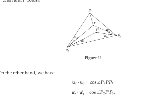
As in the classical case, the functionfPattains its absolute minimum value exactly at one point.
Theorem 3.1. Assume that conditions2.27,2.36,2.37hold. ThenfPattains its absolute min-imum value in the interior of the triangleP1P2P3at exactly one point.
We already know, byTheorem 2.7, thatfPattains its minimum at some pointPinside the triangleP1P2P3.
Arguing by contradiction, assume that the minimum is also attained at some other point
Pinside the triangle. ThenPmust lie on one of the trianglesP P1P2,P P2P3, orP P3P1possibly on one of the sidesP Pi. Assume thatPlies onP P2P3as inFigure 11.
Since we have both∇fP 0 and∇fP 0, byLemma 2.2we must have
u2·u3u2·u3 λ2
1−λ22−λ23
P1
P2
P3
P P
u2 u2
u3
u3
Figure11
On the other hand, we have
u2·u3cos∠P2P P3,
u2·u3cos∠P2PP3.
3.2
But∠P2PP3is strictly bigger than∠P2P P3, so we must have u2·u3 < u2·u3, a contra-diction.
4. Construction of the interior minimizing point
Let us assume that conditions2.27,2.36,2.37, or, equivalently, conditions2.42, are satis-fied. Then, byTheorem 2.7, there is a pointP at which the functionfPattains its minimum; moreover,Plies in the interior of the triangleP1P2P3. Also, byTheorem 3.1, this point is unique. To actually find the point, we can use a construction inspired by the one for the classical casesee, e.g.,4.
TakingP1P2as one of the sides, let us construct a triangleP1P2P3, as inFigure 12, which is similar to the triangle inFigure 4, with sidesλ1,λ2,λ3. Moreover, let us choose the angles so that the angle atP1isθ1, the angle atP2isθ2, and the angle atP3isθ3. Further, let us draw the circumcircle to this triangle, and letObe its center.
The arcP1P3P2of this circle spans the angleθ3, so the complementary arc will spanπ−θ3. Similarly, let us constructP1P2P3, also similar to the triangle with sidesλ1,λ2,λ3, as in
Figure 12, so that the angle atP1isθ1, the angle atP2isθ2, and the angle atP3isθ3. Let us also draw the circumcircle toP1P2P3, and letObe its center.
Now, the formula for the radius of the circumscribed circlesee, e.g.,1, page 13, ap-plied to the triangleP1P3P2, yields
P1P2 sinθ3
2P1O, whence P1P2
P1O
2 sinθ3. 4.1
Applying the same result to the triangleP1P3P2, we obtain P1P2
sinθ3 2P1O
, whence P1P2
P1O 2 sinθ3. 4.2
We conclude that
P1P2
P1O
P1P2
[image:11.600.101.438.81.287.2]P1
α1
P2
P3
P O
O P3
P2
θ1 θ1
θ2
θ3
π−θ3 π−θ2
θ3
θ2
Figure12
Hence, the isosceles trianglesP1OP2 andP1OP2 are similar. Therefore, the angle∠OP1P2 is equal to the angle∠OP1P2. Hence,
∠OP1O∠OP1P2∠P2P1P3∠P3P1O∠OP1P2α1∠P3P1Oα1θ1. 4.4
Now, by our assumption2.42,α1< π−θ1, whence∠OP1O< π. This guarantees that, firstly, the two circles are not tangent, and secondly, the other pointP of intersection of these circles, besidesP1, will occur inside the triangleP1P2P3. Indeed, from our construction it follows that ∠P2P P1π−θ3and∠P1P P3π−θ2. Consequently,
2π−π−θ2−π−θ2θ3θ2π−θ1, 4.5
which is less thanπ, soPcannot lie below the lineP2P3. We claim thatPis the desired minimizing point.
Indeed, geometrically, the fact that∠P2P P1 π−θ3,∠P1P P3 π−θ2, and∠P1P P3 π−θ1guarantees that atPone can arrange the vectorsλiuias inFigure 4, and therefore,
λ1u1λ2u2λ3u30, 4.6
that is,∇fP 0.
Here is an algebraic proof of the same fact. AtP, we have
∇fP2λ1u1λ2u2λ3u3
·λ1u1λ2u2λ3u3
λ21λ22λ322λ1λ2u1·u22λ1λ3u1·u32λ2λ3u2·u3
λ21λ22λ232λ1λ2cosπ−θ32λ1λ3cosπ−θ22λ2λ3cosπ−θ1 λ21λ22λ23−2λ1λ2cos θ3−2λ1λ3cos θ2−2λ2λ3cos θ1.
Now, by the cosine law,
λ21λ22−2λ1λ2cos θ3λ23, 4.8
so the above expression simplifies to
∇fP2λ23λ23−2λ1λ3 cosθ2−2λ2λ3cosθ1. 4.9
Now we add and subtractλ2
1and apply the cosine law twice again:
∇fP2 λ23λ21−2λ1λ3cosθ2
λ23−2λ2λ3cosθ1−λ21
λ22λ23−2λ2λ3cos θ1
−λ21
λ21−λ210.
4.10
Note. As for the classical case, it is not hard to show that actually the pointsP,P3, andP3 lie on the same line, and so do the pointsP, P2, and P2; this provides another geometric way of constructing the minimizing point P; see 8. Moreover, generalizing the situation in the classical case, one can see thatP3P3 d/λ3andP2P2 d/λ2, wheredis the minimum of our functionfP attained at the pointPwe just constructed.
5. Degenerate cases
Case 1. When one of the triangle inequalities2.11fails to hold then, byLemma 2.1, the ab-solute minimum cannot occur inΩ, so it must happen at one of the vertices of our triangle
P1P2P3.
Assume, for example, that
λ1≥λ2λ3. 5.1
Then, we claim that the minimum is attained atP1. Indeed, we have
fP2λ1P1P2λ3P2P3≥λ2λ3P1P2λ3P2P3λ2P1P2λ3P1P2P2P3. 5.2
By the triangle inequality, applied toP1P2P3, we haveP1P2P2P3 > P1P3. Therefore, the last expression is strictly greater than
λ2P1P2λ3P1P3f
P1
. 5.3
This shows thatfP2> fP1. One shows analogously thatfP3> fP1.
The other two possibilities of failure of2.11are discussed analogously; this leads to the following result.
Theorem 5.1. Ifλ1 ≥λ2λ3, then the absolute minimum offPis attained atP1and only atP1.
Similarly, ifλ2≥λ1λ3, the minimum is attained atP2, and ifλ3≥λ1λ2, the minimum is attained
Case 2. Assume now that the triangle inequalities2.11hold, but one of the conditions2.42
fails to hold. We claim that only one of these conditions can fail. Indeed, if we had, say, both
α1≥π−θ1,
α2≥π−θ2,
5.4
then we would have both
α1θ1≥π,
α2θ2≥π.
5.5
Adding up, we would get
α1α2
θ1θ2
≥2π, 5.6
which is impossible, sinceα1α2α3< πandθ1θ2θ3< π. So, only one of the inequalities in2.42can fail to hold.
If we have, for example,
α1≥π−θ1, 5.7
then we will have bothα2 < π−θ2andα3 < π −θ3. This implies, byLemma 2.5, the remark following it, andTheorem 2.7, that the minimum must be attained atP1.
The other two possibilities of failure of2.11are discussed similarly. The following re-sult summarizes our discussion.
Theorem 5.2. If conditions2.11hold andα1≥π−θ1,then the absolute minimum offPis attained
atP1. Similarly, ifα2≥π−θ2,then the minimum is attained atP2, and ifα3 ≥π−θ3,the minimum
is attained atP3.
6. The classical case
The classical Fermat triangle problem happens when
λ1λ2λ3. 6.1
Then, the triangles in Figures3and4are equilateral, and therefore
θ1θ2θ360◦. 6.2
Also, all the right-hand sides in2.12are equal to−1/2. Conditions2.42become
αi<120◦ fori1,2,3. 6.3
Figure13
Figure14
7. The Fermat gradient system
Assume conditions 2.42 hold. As we observed before, the gradient2.10 of the weighted distance sumfx, ygiven by2.1is defined in all ofΩ R2\ {P
1, P2, P3}. Since the function fx, yhas a global minimum at the optimal pointP, the trajectories inΩof the gradient system
x,˙ y˙ −∇fx, y 7.1
will converge to the asymptotically stable equilibriumP. This follows immediately from the fact thatVx, y −∇fx, y2is a global Lyapunov function for the system onΩ see, e.g., 10, Section 9.3. Moreover, the trajectories of7.1are orthogonal to the level curves of the weighted sumfx, y.Figure 13 illustrates the situation for a more or less randomly chosen triangle, for the classical Fermat problem, when all the weightsλi coincide. We have depicted the direction field of the gradient system plus several trajectories. The closed lines are the level curves off.
Several intriguing questions arise. For example, when the triangle is equilateral, a single level curve will be tangent to all three sides as shown inFigure 14.
it always possible to pick the weightsλiso that a single level curve off will be tangent to all three sides?
References
1 H. S. M. Coxeter, Introduction to Geometry, John Wiley & Sons, New York, NY, USA, 2nd edition, 1980. 2 R. Courant and H. Robbins, What is Mathematics?, Oxford University Press, New York, NY, USA, 1969. 3 F. Eriksson, “The Fermat-torricelli problem once more,” The Mathematical Gazette, vol. 81, no. 490, pp.
37–44, 1997.
4 R. Honsberger, Mathematical Gems. From Elementary Combinatorics, Number Theory, and Geometry, The Dolciani Mathematical Expositions, no. 1, The Mathematical Association of America, Buffalo, NY, USA, 1973.
5 M. W. Bern and R. L. Graham, “The shortest-network problem,” Scientific American, vol. 260, no. 1, pp. 84–89, 1989.
6 I. Greenberg and R. A. Robertello, “The three factory problem,” Mathematics Magazine, vol. 38, pp. 67– 72, 1965.
7 W. J. van de Lindt, “A geometrical solution of the three factory problem,” Mathematics Magazine, vol. 39, no. 3, pp. 162–165, 1966.
8 J. Tong and Y. S. Chua, “The generalized Fermat’s point,” Mathematics Magazine, vol. 68, no. 3, pp. 214– 215, 1995.
9 H. W. Kuhn, ““Steiner’s” problem revisited,” in Studies in Optimization, G. B. Dantzig and B. C. Eaves, Eds., vol. 10, pp. 52–70, The Mathematical Association of America, Washington, DC, USA, 1974. 10 M. W. Hirsch, S. Smale, and R. L. Devaney, Differential Equations, Dynamical Systems, and an Introduction