Munich Personal RePEc Archive
Trade Openness and Output Volatility
Bejan, Maria
ITAM (Instituto Tecnologico Autonomo de Mexico)
February 2006
Trade Openness and Output Volatility
∗
Maria Bejan
†February, 2006
Abstract
This paper studies the effect of trade openness on output volatility.
Wefind that trade openness generally increased output volatility, although
this effect was stronger and more significant during 1950-1975 than during
1975-2000. However, if we split the sample into developed and developing countries, we observe that more openness increased volatility in developing countries, while it helped smooth output in developed countries. We also
find that the size of the government may have increased volatility in less
developed countries. Part of the positive relation between openness and volatility may be explained by the positive relation between openness and
government size. Another important finding of this paper is that once
we control for government size and some measures of external risk, such
as terms of trade volatility and export concentration index, the effect of
openness on the output volatility turns out to be negative.
∗I am grateful to Klaus Desmet, for many comments and suggestions. First draft: October
2004
†ITAM, Av. Camino a Santa Teresa #930, Col. Héroes de Padierna, C.P. 10700 Del.
Mag-dalena Contreras, México, D.F., tel: (+52) 55 5628 4000, ext. 6531, email: [email protected]
1
Introduction
Traditionally there has been a lot of interest in the relationship between trade openness and the growth rate of output (Rodriguez and Rodrik, 1999). Less attention has been devoted to the relation between trade openness and the volatility of output. Theoretically, this relationship is not settled. On the one hand, openness leads to specialization and to more volatility if sector-specific shocks are prevalent. Also, Tornellet al (2003) shows that trade liberalization is typically followed byfinancial liberalization. But morefinancial liberalization is associated with morefinancial fragility, in the case of developing countries. Through this channel we could think that more openness (i.e. trade liberal-ization) implies more fluctuations in the GDP growth. On the other hand, trade openness may also provide a way of cushioning oneself against country-specific shocks, since the world economy as a whole is less prone to shocks than individual countries (Krebs, Krishna and Maloney, 2004). The way output volatility reacts to changes in the level of openness is an important question for a number of reasons. First, if consumption smoothing is an issue, output (and consumption) volatility may be costly in terms of welfare. Second, it has been documented that higher volatility tends to lead to lower growth (Ramey and Ramey, 1995). Third, volatility has disproportionately adverse effects on the poor countries (Easterly, Islam and Stiglitz, 2000).
We use a data set of 111 countries going from 1950 to 2000. Our mainfi nd-ings are the following. The correlation between openness and volatility tends to be positive, although it is not always significant. The correlation has become weaker over time though. Also, developing and developed countries exhibit dif-ferent patterns. Less developed countries suffer from a stronger effect of open-ness on volatility, although the effect has become weaker in recent decades. In contrast, for developed countries, the effect goes the other way: more openness smoothens output volatility. Here again the effect becomes weaker over time. The degree of specialization and the volatility of the terms of trade do a good job in explaining why openness increases output volatility. When controlling for the size of the economy, the effect of openness tends to weaken, and even disappears. Larger economies are characterized by lower output volatility. This is not surprising, as it is well known that larger countries are less prone to shocks (Head, 1995). Also richer countries display less volatility in output.
We then try to delve deeper into the role of government spending. According to Rodrik (1998), more open economies have larger governments in an attempt to deal with increased volatility. This so called ”compensation theory” claims that governments play a mitigating role on risk. In the case of developed countries, wefind evidence supporting that theory. Even after controlling for the degree of openness, government continues to reduce output volatility. However, this is no longer true for developing countries. Under some specifications, larger governments in poorer countries lead to increased volatility.
Another interesting question is how thefinancial sector affects output volatil-ity. It is often argued that opening the capital account allows risk diversification,
stabilizing, in this way, the economy. On the other hand, opening the capital account makes the country more dependent on credit, which, in turn, could make it more vulnerable. Easterly, Islam and Stiglitz (2000) show thatfinancial depth, measured by private credit to GDP, affects output volatility in a non-monotonic way: initially it tends to decrease volatility but too much private credit ends up increasing output volatility. Also they do notfind any evidence for the stabilizing role of capitalflows. On the other hand, Svaleryd and Vlachos (2000) found a positive relationship between openness to trade and development offinancial markets, measured by proxies like liquid liabilities and credit to pri-vate enterprises. So it is interesting to see how much of the effect of openness on output volatility is attributed to the development offinancial markets. To inves-tigate that, we introduced in our analysis somefinancial proxies such as black market premium, foreign debt, credit to private sector and liquid liabilities. Our results show that among thesefinancial proxies only the black market premium plays a role in explaining output volatility. In all but the developed economies sample, the black market premium passed from being insignificant during the period 1950-1975 to being highly significant over 1975-2000. Moreover a higher average level of black market premium seems to increase output volatility while a higher variability in the black market premium helps smoothing the volatility of output.
The paper is organized as follows. In the next section we describe the data and present some simple regressions that give a first insight into how open-ness affects volatility of output. Section 3 includes some robustness tests of the relationship between openness and volatility and presents the reasons for including each variable into our regressions. This is followed by the presenta-tion of the results and a possible interpretapresenta-tion of them. Secpresenta-tion 4 presents the government-volatility relationship. In the last section we summarize the results and make some suggestions for future research.
2
A
fi
rst look at the data
The data in this study comes from the Penn World Tables 6.1, the Inter-national Monetary Fund, the World Bank and UNCTAD. We use a sample of 111 countries over the period 1950-2000. A detailed description of the data set is presented in the Appendix 4. We start by running some simple regressions of output volatility on the level of openness for the entire set of countries. Then we will split the sample into developed and developing countries, and also check whether the effect of openness on output volatility changed over time. For that, we consider two different time periods (1950-1975 and 1975-2000).
last measure is that an economy which grows at a high but constant rate would nevertheless display high volatility. We prefer a measure which is not sensitive to growth in that way. For openness, we focus on the traditional measure:
openness=imports+exports
GDP (%)
To just give an example, take the case of Mauritania and the United States. Mauritania, with an openness level of 87.87 is 6.4 times more open than the United States, with an openness level of 13.66. This big difference in the level of openness corresponds to a difference of 0.100 in the volatility of output (0.025 in the United States and 0.125 in Mauritania). This, in relative terms, means that Mauritania is 5 times more volatile than the United States. Therefore this case seems to sustain the idea that more openness implies more output volatility. Nevertheless this is just an example. The objective of this paper is to dig deeper into the data and investigate if this hypothesis is, in fact, a more general and robust result.
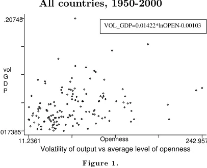
All countries, 1950-2000
vol
G
D
P
Volatility of output vs average level of openness
Openness
11.2361
242.957
.017385 .20745
[image:5.595.207.410.324.489.2]VOL_GDP=0.01422*lnOPEN - 0.00103
Figure 1.
Figure 1 plots output volatility as a function of openness for the time pe-riod 1950-2000, using the entire sample of 111 countries. As one can see from the picture, there is a positive relationship between openness and volatility of output: more open economies exhibit higher output volatility. A simple regres-sion shows that, on average, an increase of 10% in openness increases output volatility by 0.0015. This relation is significant at the 99% level.
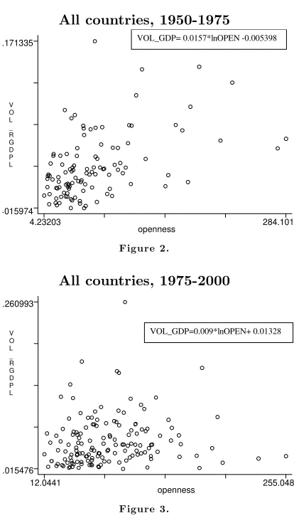
All countries, 1950-1975
V
O
L
_
R
G
D
P
L
openness
4.23203
284.101
.015974
.171335
[image:6.595.204.411.116.480.2]VOL_GDP= 0.0157*lnOPEN - 0.005398
Figure 2.
All countries, 1975-2000
V
O
L
_
R
G
D
P
L
openness
12.0441
255.048
.015476
.260993
VOL_GDP=0.009*lnOPEN+ 0.01328
Figure 3.
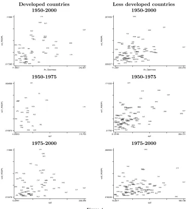
For the sample of developed1 countries, the relation between openness and
output volatility is significant for the entire period (1950-2000) but not for the two subperiods (1950-1975 and 1975-2000). For the sample of developing countries, the coefficient of openness on output volatility decreases over time and also becomes less significant. Figure 4 shows the relationship between openness and volatility of output for developed and developing countries subsamples.
As we can see from the graphs, the positive relationship does not disappear if we split the sample. However, if we analyze the data set in more detail we observe that countries like the United States and Belgium, with completely different trade regimes, display similar degrees of volatility. The United States is a relatively closed economy with an openness index of 13.66 compared to Belgium, where the openness level is 90.42. Over the period 1950-2000 they display very similar degrees of volatility: 0.024 in USA versus 0.020 in Belgium.
1We call a developed country any country that has the average level of GDP per capita
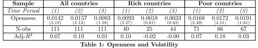
This gives us an idea that the relationship between openness and volatility is not as trivial as it might be thought. Moreover, inTable 1 we could observe that in the case of developed countries the relationship is significant only if we consider the entire period of time but it disappears when we split the time period. In the case of less developed economies we have the same effect as in the pooled sample (i.e. with all the countries together). Not only does the coefficient of openness decrease over time, but its significance also decreases from the 99% level before 1975 to only 90% after 1975.
Developed countries Less developed countries
1950-2000 v o l_ RG DP L Av_Openness 11.6657 242.957 .017385 .11869 ATG ARG AUS AUT BRB BLR BEL BGR CAN CUB CYP CZE DNK EST FIN FRA GAB DEU GRC HKG HUN ISL IRL ISR ITA JPN KAZ LVA LUX MAC MUS MEX NLD NZL NOR POL PRT PRI SYC SGP SVK SVN ZAF ESP LCA SWE CHE TTO USA UKR GBR URY VEN 1950-2000 v o l_ RG DP L Av_Openness 11.2361 235.016 .020227 .207459 ALB DZA AGO ARM AZE BGD BLZ BEN BOL BWA BRA BFA BDI CMR CPV CAF TCD CHL CHN COL CRI CIV DMA DOM ECUEGY SLV GNQ ETH FJI GMB GHA GRD GTM GIN GNB GUY HTI HND IND IDN IRN JAM JOR KEN LBN LSO MDG MWI MYS MLI MRT MAR MOZ NAM NPL NIC NER NGA PAK PAN PNG PRY PER PHL ROM RWA STP SEN SLE LKA KNA VCT SYR TWN TZA THA TGO TUN TUR UGA ZMB ZWE 1950-1975 v o l1_RG D PL op1 4.23203 170.703 .015974 .064666 ARG AUS AUT BEL CAN DNK FIN FRA DEU HUN ISL IRL ISR ITA JPN LUX NLD NZL NOR ESP SWE CHE USA GBR VEN 1950-1975 v o l1_RG D PL op1 8.16156 284.101 .01793 .171335 DZA AGO BGD BRB BEN BOL BWA BRA BFA BDI CMR CPV CAF TCD CHL CHN COL CRI CIV CYP DOM ECUEGY SLV GNQ ETH FJI GAB GMB GHA GRC GTM GIN GNB GUY HTI HND HKG IND IDN IRN JAM JOR KEN LSO MDG MWI MYS MLI MRT MUS MEX MAR MOZ NAM NPL NIC NER NGA PAK PAN PNG PRY PER PHL POL
[image:7.595.145.518.238.655.2]3
Robustness
The results above are nothing more than a first cut at the data. Clearly it is necessary to control for other effects which could have an impact on volatility before jumping to the conclusion that greater openness leads to higher output volatility. The existing literature has identified a number of other sources of output volatility. In this section we start by summing up those other possible explanatory variables. We then analyze whether the positive relation between openness and output volatility is preserved once we include those control vari-ables.
3.1
Control variables
We now give a list of all the control variables we use in our regressions, and explain why they might have an effect on output volatility.
• Country size and development
The way one country reacts to any shock depends on some basic charac-teristics such as the size and the level of development. The most common proxies used to measure these features are the population and the level of GDP per capita. A number of cross-section analyses trying to explain out-put volatility use GDP per capita and population as control variables and most of the time they turn out to be significant (see for example Easterly, Islam and Stiglitz (2000), Mobarak (2004), Tamirisa (1999), Wolf (2003), Wu and Rapallo (1997)). Regarding the influence of these variables on the output volatility, we expect a country with a higher level of GDP per capita (or larger population) to exhibit lowerfluctuations.
• Government expenditure
As argued by Rodrik (1996), government plays a risk-reducing role in economies exposed to external risk by providing social insurance. There-fore we would expect a negative influence of government expenditure on output volatility in our analysis.
• Human capital
Mobarak (2004) and Wolf (2003) used the average level of human capi-tal as a control variable to explain the observed volatility in output and consumption. Both of them found that a country with a higher level of human capital can better adapt to new situations, therefore its output and consumption are less affected by a shock. We should therefore expect, in our analysis, a country with a higher level of human capital to display less volatility in its GDP per capita.
• Financial markets proxies
markets. We would expect a more developed financial system to reduce output volatility. Svaleryd and Vlachos (2002), in their empirical study of the relationship between openness and markets for risk, classify proxies forfinancial development into three categories: the size offinancial sector (ratio of liquid liabilities to GDP), thefinancial system’s ability to allocate credit (credit issued to private sector, divided by GDP) and thereal interest rate. They found evidence that all these proxies have a positive and strong influence on the level of openness of a country. Lee (1993), using theblack market premium as a proxy for capital and exchange controls, found that these controls tend to reduce trade. These are the reasons to think that there could be a strong impact of these proxies on output volatility too.
• Foreign direct investment (FDI)
FDI generates some links between production processes across countries. Atfirst sight, one may think that this provides a way to alleviate country specific shocks and thus decrease output volatility. However, Barrell and Gottschalk (2004) test this hypothesis for the cases of US and UK and
find that the effect of FDI on output volatility is not significant. We also want to test this hypothesis in our cross-section analysis.
• Total investment
Investment plays a central role in output growth through the rate of return on capital and the process of capital accumulation. Ramey and Ramey (1995) show that investment has a strong negative effect on the volatility of GDP and we would expect the same relationship in our analysis: a country with a higher level of investment should display less volatility in its output.
• Inflation
Financial volatility could be an important factor affecting output volatility of an economy. Many papersfind that inflation volatility has an important positive effect on consumption volatility (Wolf (2003), Wu and Rapallo (1997)). Old Phillips curve models imply a permanent trade-offbetween inflation and output. We would therefore expect to have a positive impact of the volatility of inflation on output volatility.
• External risk proxies
volatility of terms of trade, Rodrik found that the openness coefficient turns out to be insignificant. This highlights the fact that the volatility of the terms of trade is the channel through which openness affects the size of the government. In the light of these findings, we expect to obtain a positive influence of the terms of trade volatility on output volatility and the openness effect to disappear.
• Geographical dummies
The relationship between openness and volatility could be affected by a common factor that affects both variables. Geographical dummies are standard candidates (see for example Mobarak (2004), Razin and Rose (1992), Rodrik (1998), Svaleryd and Vlachos (2002)).
3.2
Empirical results for the pooled sample
We start by looking at the entire sample of countries. Table 2 reports the results for the time period 1950-2000, whereasTables 3 and 4 look at the subperiods 1950-1975 and 1975-2000. The number of control variables for the second subperiod is greater, because of better data availability. Openness tends to have a positive and significant effect on output volatility. This effect was both greater and more significant in the period 1950-1975 than in the period 1975-2000. If during the period 1950-1975 a 10% increase in the level of openness would mean a 0.0015 increase in the volatility of output, over the period 1975-2000 this impact decreases to only 0.0001. Moreover, if we pay attention to the adjustedR2 as a measure of how the equationsfit the reality, we can observe a
decrease over time in all the equations.
From the same tables we can observe that the control variables are always significant and tend to have the expected sign: GDP per capita, human capital, the level of investment and FDI inflows decrease volatility, whereas inflation increases volatility. We also observe that regional dummies do not seem to have any effect on the volatility of output.
As reported inTable 4, once we control for the export concentration index, openness ceases to have a positive effect on volatility. We could only check for this effect during the period 1975-2000, because earlier data was insufficient. The result from this table seems to suggest that openness increases volatility because openness leads to greater specialization, making the economy more vulnerable to external (sectoral) shocks. This specification is also the one with the highest adjustedR2among all the regressions for the second period of time.
6 and 7. In nearly all regressions both GDP per capita and population have a negative and significant effect on volatility. There is also a marked improvement in the adjustedR2, suggesting that these two variables have high explanatory
power. The effect of openness on volatility becomes smaller — even negative— and less significant. Whereas for the time period 1950-1975 openness continues to be statistically significant, this is no longer true for the period 1975-2000. During the period 1975-2000 we observe a negative effect of openness on volatility but this effect does not result to be significant at the 90% level. The main results are therefore confirmed: openness tends to increase volatility, but much less – or even not at all – in recent decades. As far as the other explanatory variables are concerned, they tend to lose significance, once we include GDP per capita and population. Only inflation continues to increase volatility and FDI inflow continues to smooth output over 1950-1975. These effects disappear over time, though. During the second period, 1975-2000, only volatility in the terms of trade results to have a significant positive influence on output volatility. As before, this suggests that openness may increase output volatility because of a higher exposure to external shocks. Introducing geographical dummy variables does not improve results.
Another interesting question is to see whether the degree of trade openness is proxying for the degree of openness offinancial markets. As for the proxies for
financial development (seeTables 8, 9 and10), only the black market premium, foreign debt and liquid liabilities increase the explicative power of the regressions in the second period of time. From these control variables only black market premium is significant per se. We observe that a higher average level of black market premium increases output volatility while more variability in the level of black market premium smooths the volatility of GDP. An interesting issue here is that the effect of black market premium on output volatility becomes stronger over time while the opposite happens with the openness effect. This fact could suggest that maybe trade openness is simply picking upfinancial openness.
3.3
Empirical results for the developed countries
During the period 1950-1975 inflation proved to have a strong effect in raising volatility of output while over the next period its role was replaced by the volatility in terms of trade and export concentration index, which explain more than half of the volatility displayed by GDP. Another aspect presented inTables 11-18 is the effect of GDP per capita, which becomes highly significant only in the second period, and population, which increases its significance during 1975-2000. The regional dummies’ lack of effect on volatility is still present in the case of developed economies.
Tables 13 and 14 present the effect of financial development proxies on volatility in output in the case of developed countries. As in the pooled sam-ple, none of these variables affects volatility in the first period but this ”zero-influence” is still present during the second period in the case of rich countries. The only effect they have is to decrease the significance of the openness coeffi -cient. Taking a look at theR2-s we observe that controlling forfinancial proxies
in the case of rich economies does not help improve the explanatory power of the regressions.
3.4
Empirical results for the developing countries
The results for the sample of developing countries are reported inTables 15 to
18. There, like in the case of the entire sample, the highest level of significance for openness is reached in thefirst subperiod of time. Moreover, we see that the effect of openness does not disappear once we control for the population size and GDP per capita (see Table 1 andTables 15, 16). Like in the case of the total sample the combination openness, GDP, population and inflation explains almost half of the variability in the GDP growth over the period 1950-1975. If we take a look at Table 16 we observe that during the period 1975-2000 the European location seems to be the only one that affects output volatility in poor countries. Also comparingTables 15 and 16 we observe that, in terms of the explanatory power, inflation’s role in thefirst period is replaced by that of the volatility in terms of trade in the second period. In terms offinancial market accessibility (Tables 17 and 18), in the first subperiod we do not see any influence of thefinancial proxies on volatility. In the second subperiod, we see the same influence of the black market premium for the pooled sample. The openness effect on output volatility is replaced by the black market premium effect.
4
Government, Openness and Volatility
spending. This is called the ”compensation theory” and it received empirical support in Rodrik’s paper for a broad sample of countries. However, in a recent study of OECD countries, Molana, Motagna and Violato (2004) claim that this theory only holds for a limited number of countries.
The question we address in this section is slightly different: when controlling for openness, does government spending continue to have a mitigating effect on volatility? Table 19 shows the results of the regression of output volatility on openness and government spending, distinguishing between different time pe-riods and splitting up the sample into rich and poor countries. For the entire sample of countries, openness increases output volatility, and government size decreases output volatility. This seems to reinforce the view of Rodrik (1998): for a given level of openness, bigger governments reduce output volatility. How-ever, splitting the sample into developed and less developed countries we see that the government size effect disappears in the case of less developed economies.
Table 20 presents the results of the same exercise when we controlled for the level of GDP per capita and population. Once we do that, the mitigating effect of government spending on output volatility still appears only in the richer coun-tries, over the period 1975-2000. In fact, for the entire sample of countries and for the poorer countries, government spending now increases output volatility, although the effect is not significant.
government which, in turn, can compensate for the negative effects of shocks. In conclusion, more openness means less volatility of output. In the poor coun-tries not only can we not say the same, but the role played by the government is completely different: more government expenditure increases output volatil-ity and this effect remains strongly significant and positive irrespective of the proxies for external shocks we add.
5
Conclusions
This paper has explored the relationship between trade openness and out-put volatility. We have found that this relationship is a complex one. In devel-oping countries more openness is associated with higher volatility. In contrast, in developed countries openness smoothens output volatility. However, for both samples the relationship has become weaker in recent decades.
An interesting feature we found in the case of developing countries is that the decreasing effect over time of openness on trade is associated with an increasing effect of the black market premium (as a proxy for financial development) on output volatility. This fact could suggest that maybe trade openness is partly picking upfinancial openness.
6
Bibliography
• ANDERSON, H.M.; KWARK, N., VAHID, F.: ”Does International Trade
Synchronize Business Cycles?”,Monash University Working Paper8 (1999)
• BARRELL, R., GOTTSCHALK, S.: ”The Volatility of the Output Gap
in the G7”,NIESR Working Paper (2004)
• BREEN,R., PENALOSA,C.: ”Income Inequality and Macroeconomic Volatil-ity”, forthcoming: Review of Development Economics
• EASTERLY, W., ISLAM, R. and STIGLITZ, J.: ”Explaining Growth
Volatility”,World Bank Working Paper (2000)
• HARRISON, A.: ”Openness and Growth: A time-series cross-country
analysis for developing countries”, Journal of Development Economics
(1996)
• Head, A.C., ”Country Size, Aggregate Fluctuations and International Risk Sharing”Canadian Journal of Economics, 28(4b) (1995)
• IMBS, J.:”Why the Link Between Volatility and Growth is Both Positive and Negative”,CEPR Working Paper (2002)
• JEREMY, D.: ”International Technology Transfer : Europe, Japan and the USA, 1700-1914” ,Aldershot : Edward Elgar (1991)
• KRAAY, A., VENTURA, J.: Trade Integration and Risk Sharing”,World Bank Working Paper, February (2002)
• KORMENDI, R.C., MEGUIRE, P.G.: ”Macroeconomic Determinants of
Growth (Cross-Country Evidence)”, Journal of Monetary Economics 16 (1995)
• KREBS,T.,KRISHNA, P., MALONEY, B.: ”Trade Policy, Income Risk,
and Welfare”,Brown University Working Paper (2004)
• LEE, J.W.: ”International Trade, Distortions and Log-Run Economic Growth”,IMF Staff Papers no 40 (1993)
• LEVINE, R. and RENELT, D.:”A Sensitivity Analysis of Cross-Country Growth Regressions”,World Bank Staff Paper (1992)
• MOBARAK, A.M.: ”Determinants of Volatility and Implications for Eco-nomic Development”, Forthcoming (The Review of Economics and Sta-tistics)
• MOLANA,H., MONTAGNA,C., VIOLATO,M.: ”On the Causal
• RAMEY, G., RAMEY, V.: ”Cross-Country Evidence on the Link Between Volatility and Growth”,The American Economic Review, December 1995
• RAZIN, A., ROSE, A.: ”Business Cycle Volatility and Openness: An Exploratory Cross-Section Analysis”, NBER Working Paper No. 4208 (1992)
• RODRIK, D.: ”Why Do More Open Economies Have Bigger
Govern-ments?”,Journal of Political Economy, 106(5) (1998)
• RODRIK, D., RODRIGUEZ, F.: ”Trade Policy and Economic Growth: A
Skeptic’s Guide to the Cross-National Evidence”,NBER Working Paper
No. 7081 (1999)
• SVALERYD, H., VLACHOS, J.: ”Markets for Risk and Openness to
Trade: How Are They Related”, Journal of International Economics, 57(2000)
• TAMIRISA, N.: ”Exchange and Capital Controls as Barriers to Trade”,
IMF Staff Papers (1999)
• TORNELL, A., WESTERMANN, F., MARTINEZ, L.: “Liberalization,
Growth and Financial Crises: Lessons from Mexico and the Developing World”,Brookings Papers on Economic Activity No. 2 (2003)
• WOLF, H.:”Accounting for Consumption Volatility Differences”,IMF Staff
Papers 51(2004)
• WU, C.H., RAPALLO, P.: ”Macroeconomic determinants of output growth volatility: a cross-country regression analysis 1961-1988”,Working Paper University of California, San Diego (1997)
7
Appendix 1: Data Description
In this appendix we will describe in detail the variables we use and the sources we took them.
• volatility=standard deviation of the growth rate of real GDP per capita in constant prices: Laspeyres index (Penn World Tables 6.1) (1950-2000)
• OPEN=average level of openness ((imports+exports) as percentage of GDP) (1950-2000) (Penn World Tables 6.1)
• total GDP=log of the average level of GDP Laspeyres index (1950-2000) (Penn World Tables 6.1)
• GDP per capita=log of the average level of GDP per capita Laspeyres index (1950-2000) (Penn World Tables 6.1)
• population=log of the average level of population (1950-2000) (Penn World Tables 6.1)
• human capital=average level of human capital (Barro & Lee data 1960-2000: average years of school)
• FDI inflow=log of the average FDI (foreign direct investment) inflow (1970-2000) (IMF-IFS: International Monetary Fund-International Finan-cial Statistics)
• investment=log of the average investment (1950-2000) (Penn World Tables 6.1)
• government=log of the average level of government expenditure (1950-2000) (Penn World Tables 6.1)
• export index=export concentration index (averaged 1980-2000) (UNC-TAD Handbook of Statistics)
This is a modified version of the Herfindahl-Hirschman index:
Hi=
s
239P
i=1
(Eij
Ei.)
2−q 1
239
1−q2391
whereHi=concentration index for country i,Eij=value of export of productj
and countryi,Ei.=
239P
j=1
Eij
• terms of trade=standard deviation of the terms of trade (1980-2000) (UNC-TAD Handbook of Statistics)
• inflation=standard deviation of inflation (1950-2000) (consumption price index: Penn World Tables 6.1)
• black market premium av=black market premium average level (exchange rate in the black market, divided by the official rate) (average 1960-1999) (”Global Development Network Growth Database”, Easterly & Sewadeh, World Bank)
• interest rate= standard deviation of the national interest rate (IMF-IFS) (1950-2000)
• liquid liabilities=average liquid liabilities % GDP (IMF-IFS) (1950-2000)
• credit to private sector=average credit to private sector % GDP (IMF_IFS) (1950-2000)
8
Appendix 2: Tables
.
Sample All countries Rich countries Poor countries
Time Period (1) (2) (3) (1) (2) (3) (1) (2) (3)
Openness 0.0142
(3.19) 0(5.0157.12) 0(1.0093.58) 0(2.0093.27) 0(0.0018.61) 0(0.0033.82) 0(2.0168.49) 0(4.0172.51) 0(1.0191.81)
N-obs 111 111 111 40 25 44 71 86 67
[image:19.842.136.570.132.213.2]Adj-R2 0.07 0.19 0.01 0.10 -0.02 -0.00 0.07 0.18 0.03
Table 1: Openness and Volatility
N= nr of observations, t-statistics in parenthesis
(1) all the interval:1950-2000(2)1st subperiod: 1950-1975,(3)2nd subperiod: 1975-2000
8.1
The entire sample (all countries)
Time Period 1950-2000
Openness 0.0142
(3.19) 0(3.0129.25) −(−0.00025.53) 0(0.0054.96) 0(3.0138.43) 0(3.0109.35) 0(3.0138.37) 0(2.0072.09) 0(2.0103.41)
GDP per capita −0.0137
(−5.27)
Total GDP −0.0095
(−5.88)
Population −0.0053
(−2.46)
Investment −0.009
(−5.00)
Human Capital −0.0032
(−4.08)
Inflation 0.1467
(4.51)
FDI Inflow −0.0050
(−5.28)
Europe −0.0085
(−0.57)
Africa 0.0263
(1.84)
Asia 0.0053
(0.35)
North America −0.0011
(−0.08)
South America 0.0055
(0.35)
N-obs 111 111 111 111 111 92 111 91 111
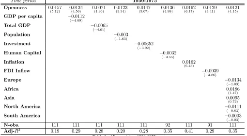
[image:19.842.140.633.270.558.2]Time period 1950-1975
Openness 0.0157
(5.12) 0(4.0134.56) 0(1.0071.96) 0(3.0123.34) 0(5.0147.07) 0(4.0136.99) 0(6.0162.17) 0(4.0129.41) 0(4.0121.15)
GDP per capita −0.0112
(−4.09)
Total GDP −0.0065
(−4.01)
Population −0.003
(−1.63)
Investment −0.00652
(−3.92)
Human Capital −0.0032
(−3.55)
Inflation 0.0162
(6.43)
FDI Inflow −0.0039
(−3.86)
Europe −0.0134
(−1.03)
Africa 0.0186
(1.47)
Asia 0.0095
(0.72)
North America −0.0111
(−0.83)
South America −0.0003
(−0.03)
N-obs. 111 111 111 111 111 92 111 91 111
[image:20.842.147.657.101.381.2]Adj-R2 0.19 0.29 0.28 0.20 0.28 0.35 0.41 0.29 0.35
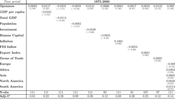
Time period 1975-2000
Openness 0.0093
(1.58) 0(2.0117.22) −(0−.10101.71) −(0−.00058.78) 0(2.0121.26) 0(1.0066.53) 0(1.0083.46) 0(0.0017.41) 0(0.0016.38) 0(2.0132.15) 0(1.008.40)
GDP per capita −0.0161
(−5.53)
Total GDP −0.0114
(−6.43)
Population −0.0082
(−3.15)
Investment −0.0108
(−5.09)
Human Capital −0.0031
(−3.45)
Inflation 0.1065
(3.08)
FDI Inflow −0.0054
(−4.88)
Export Index 0.0681
(5.80)
Terms of Trade 0.0005
(3.32)
Europe −0.008
(−0.43)
Africa 0.0294
(1.64)
Asia 0.0005
(0.03)
North America 0.0048
(0.25)
South America 0.0114
(0.57)
N-obs 111 111 111 111 111 92 111 91 107 97 111
[image:21.842.156.719.97.415.2]Adj-R2 0.01 0.22 0.28 0.09 0.20 0.12 0.08 0.20 0.25 0.12 0.14
Time Period 1950-2000
Openness 0.00158
(0.32) 0.(000019.04) 0(1.0052.30) 0(0.0028.60) 0(0.0042.90) −(0−.00003.07)
GDP per capita −0.0149
(−5.98) −(−0.20229.66) −(0−.20097.28) −(0−.50127.15) −(0−.20111.22) −(0−.20107.90)
Population −0.0068
(−3.60) −(−0.30073.72) −(0−.20034.20) −(−03.006.28) −(0−.10034.29) −(0−.30072.39)
Investment 0.0056
(0.97)
Human Capital −0.0004
(−0.30)
Inflation 0.099
(3.31)
FDI Inflow −0.0008
(−0.36)
Europe 0.0023
(0.17)
Africa 0.0158
(1.09)
Asia 0.0125
(0.84)
North America −0.0013
(−0.09)
South America 0.0038
(0.26)
N-obs 111 111 92 111 91 111
[image:22.842.148.530.116.382.2]Adj-R2 0.33 0.33 0.30 0.39 0.31 0.33
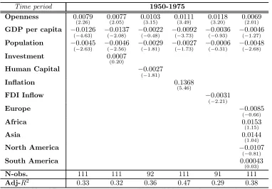
Time period 1950-1975
Openness 0.0079
(2.26) 0(2.0077.05) 0(3.0103.15) 0(3.0111.49) 0(3.0118.20) 0(2.0069.01)
GDP per capita −0.0126
(−4.63) −(−0.20137.08) −(0−.00022.48) −(0−.30092.73) −(0−.00036.93) −(0−.10046.27)
Population −0.0045
(−2.63) −(−0.20046.56) −(0−.10029.81) −(0−.10027.73) −(0−.00006.31) −(0−.20048.68)
Investment 0.0007
(0.20)
Human Capital −0.0027
(−1.81)
Inflation 0.1368
(5.46)
FDI Inflow −0.0031
(−2.21)
Europe −0.0085
(−0.66)
Africa 0.0153
(1.15)
Asia 0.0144
(1.04)
North America −0.0107
(−0.81)
South America 0.00043
(0.03)
N-obs. 111 111 92 111 91 111
[image:23.842.148.530.93.359.2]Adj-R2 0.33 0.32 0.36 0.47 0.29 0.38
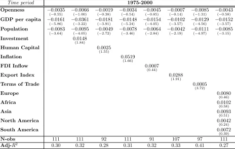
Time period 1975-2000
Openness −0.0035
(−0.55) −(−0.10066.00) −(0−.00019.38) −(0−.00034.54) −(0−.00045.85) −(−0.00007.14) −(0−.10085.31) −(0−.00043.58)
GDP per capita −0.0161
(−5.86) −(−0.30361.22) −(0−.30181.91) −(0−.50148.24) −(0−.40154.05) −(−0.30102.57) −(0−.40129.56) −(0−.30152.57)
Population −0.0083
(−3.64) −(−0.40095.05) −(0−.20049.72) −(0−.30078.46) −(0−.20064.84) −(−0.20042.19) −(0−.40111.97) −(0−.30085.15)
Investment 0.0148
(1.84)
Human Capital 0.0025
(1.55)
Inflation 0.0519
(1.66)
FDI Inflow 0.0007
(0.44)
Export Index 0.0288
(1.91)
Terms of Trade 0.0005
(3.72)
Europe 0.0080
(0.46)
Africa 0.0102
(0.58)
Asia 0.0093
(0.51)
North America 0.0042
(0.24)
South America 0.0072
(0.39)
N-obs 111 111 92 111 91 107 97 111
[image:24.842.154.618.97.391.2]Adj-R2 0.30 0.32 0.28 0.31 0.32 0.33 0.41 0.27
Time Period 1950-2000
Openness −0.0005
(−0.11) 0.(000306.40) −(−0.00025.38) 0(0.0030.67) 0(0.0033.67)
GDP per capita −0.0120
(−5.09) −(0−.012223.70) −(−0.40138.80) −(−0.50122.42) −(−0.50140.30)
Population −0.0068
(−3.33) −(−0.20057.11) −(−0.20062.82) −(−0.30055.11) −(−03.007.12)
Black Market Premium Av. 0.00015
(3.46)
Black Market Premium Vol. −0.00003
(−3.24)
St. dev of Interest Rate 0.00005
(0.40)
Foreign Debt 4.47E−16
(0.95)
Credit to Private Sector 7.97E−16
(0.76)
Liquid Liabilities 0.000
(1.00)
N-obs 92 43 36 93 73
[image:25.842.149.578.94.303.2]Adj-R2 0.37 0.33 0.44 0.34 0.36
Time Period 1950-1975
Openness 0.0065
(1.56) 0(0.0019.39) −(−0.10074.30) 0.(200891.25) 0(2.0111.38)
GDP per capita −0.0113
(−3.66) −(0−.20097.91) −(−0.40173.29) −(0−.30101.25) −(0−.20094.56)
Population −0.0047
(−2.12) −(0−.10034.45) −(−0.30091.53) −(0−.20046.35) −(0−.10049.85)
Black Market Premium Av. −0.0000
(−0.50)
Black Market Premium Vol. 8.84E−06
(0.40)
St. dev of Interest Rate −0.0060
(−1.50)
Foreign Debt 2.77E−11
(0.94)
Credit to Private Sector 2.04E−14
(0.46)
Liquid Liabilities 0.000
(1.08)
N-obs 92 43 36 93 73
[image:26.842.149.582.94.306.2]Adj-R2 0.25 0.32 0.40 0.28 0.25
Time Period 1975-2000
Openness −0.0034
(−0.56) 0(0.0068.59) 0(0.0034.48) −(0−.10057.04) −(0−.10065.12)
GDP per capita −0.0120
(−4.73) −(0−.30128.55) −(−0.50127.17) −(0−.50134.90) −(0−.60160.20)
Population −0.006
(−2.71) −(0−.10064.83) −(−0.10038.81) −(0−.30071.53) −(0−.30090.67)
Black Market Premium Av. 0.0001
(3.12)
Black Market Premium Vol. −0.00003
(−2.93)
St. dev of Interest Rate 0.0001
(0.77)
Foreign Debt 2.23E−16
(0.61)
Credit to Private Sector 1.72E−16
(0.29)
Liquid Liabilities 0.00002
(1.14)
N-obs 92 43 36 93 73
[image:27.842.149.573.94.303.2]Adj-R2 0.32 0.30 0.44 0.33 0.40
8.2
Developed countries
Time period 1950-1975
Openness −0.0094
(−2.10) −(0−.20094.06) −(0−.20106.12) −(−0.00036.89) −(−0.30227.19) −(−0.10064.54)
GDP per capita −0.0108
(−1.34) −(−0.10159.18) −(0−.00065.59) 0(0.0000.01) −(−0.00079.91) −(−0.00045.52)
Population −0.0071
(−3.12) −(0−.20069.89) −(0−.20075.97) −(−0.10037.68) −(−0.30130.89) −(−0.30065.14)
Investment 0.0050
(0.48)
Human Capital −0.0014
(−0.81)
Inflation 0.1299
(3.25)
FDI Inflow 0.0027
(1.46)
Europe −0.0079
(−1.04)
Asia 0.0110
(1.03)
North America −0.0031
(−0.31)
South America 0.0095
(0.94)
N-obs. 25 25 23 25 21 25
[image:28.842.146.509.127.371.2]Adj-R2 0.26 0.23 0.22 0.49 0.44 0.44
Time period 1975-2000
Openness −0.0053
(−1.29) −(−0.00041.97) −(0−.10052.43) −(0−.00014.31) −(0−.10049.31) −(−0.00038.98) −(−01..00630) −(0−.10060.19)
GDP per capita −0.0227
(−4.50) −(−0.00065.47) −(0−.30236.76) −(0−.30201.91) −(0−.30188.81) −(−0.20154.81) −(0−.10100.42) −(0−.20151.32)
Population −0.0064
(−3.91) −(−0.30056.24) −(0−.30054.97) −(0−.20049.77) −(0−.30055.57) −(−0.20035.00) −(0−.40081.31) −(0−.30063.41)
Investment −0.0121
(−1.25)
Human Capital 0.0011
(0.86)
Inflation 0.0868
(1.74)
FDI Inflow 0.0000
(0.06)
Export Index 0.0487
(2.91)
Terms of Trade 0.00033
(2.69)
Europe 0.0053
(0.50)
Africa 0.0201
(1.49)
Asia 0.0094
(0.74)
North America 0.0193
(1.59)
South America 0.0149
(1.14)
N-obs 44 44 40 44 37 43 34 44
[image:29.842.159.615.96.393.2]Adj-R2 0.47 0.48 0.50 0.49 0.47 0.56 0.57 0.49
Time Period 1950-1975
Openness −0.0087
(−1.37) −(−0.00069.80) −(−0.10137.76) −(−0.20106.03) −(0−.10068.48)
GDP per capita −0.0074
(−0.72) −(−0.00179.94) −(−0.10223.41) −(−0.00096.93) −(0−.10183.93)
Population −0.0066
(−0.87) −(−0.10064.57) −(−0.20094.35) −(−0.20073.74) −(0−.30078.78)
Black Market Premium Av. 0.00002
(0.39)
Black Market Premium Vol. 0.00008
(0.56)
St. dev of Interest Rate 0.0127
(1.08)
Foreign Debt 9.77E−10
(0.03)
Credit to Private Sector 1.61E−16
(0.01)
Liquid Liabilities 3.42E−06
(0.64)
N-obs 22 10 12 22 17
[image:30.842.149.580.94.303.2]Adj-R2 0.09 -0.05 0.42 0.20 0.47
Time Period 1975-2000
Openness −0.0048
(−0.90) 0(0.0142.62) −(0−.00005.09) −(−0.10059.18) −(0−.00055.95)
GDP per capita −0.0200
(−3.03) −(−0.20364.31) −(−0.30163.04) −(−0.30237.88) −(0−.30243.23)
Population −0.0067
(−2.70) −(−0.00034.61) −(−0.10025.44) −(−0.30067.62) −(0−.20078.96)
Black Market Premium Av. 0.0003
(0.56)
Black Market Premium Vol. −0.0002
(−0.47)
St. dev of Interest Rate −0.0019
(−1.52)
Foreign Debt 5.25E−11
(0.24)
Credit to Private Sector 1.03E−15
(0.23)
Liquid Liabilities 0.00001
(1.38)
N-obs 34 13 15 37 26
[image:31.842.152.575.93.305.2]Adj-R2 0.36 0.44 0.43 0.48 0.38
8.3
Less developed countries
Time period 1950-1975
Openness 0.0119
(2.87) 0(2.0119.66) 0(3.0140.73) 0(4.0148.00) 0(3.0149.51) −(−0.00069.55)
GDP per capita −0.0122
(−2.73) −(0−.10123.51) −(0−.00007.12) −(−0.20103.63) −(−0.00002.04) −(−0.10154.80)
Population −0.0050
(−2.45) −(0−.20050.31) −(0−.10029.49) −(−0.10035.95) −(−0.00008.34) −(−0.30149.42)
Investment 0.0001
(0.02)
Human Capital −0.0037
(−1.81)
Inflation 0.1394
(4.95)
FDI Inflow −0.0029
(−1.74)
Europe 0.0144
(0.66)
Africa 0.0189
(1.01)
Asia 0.0232
(1.17)
North America −0.0082
(−0.43)
South America 0.0079
(0.39)
N-obs. 86 86 69 86 70 86
[image:32.842.146.509.127.390.2]Adj-R2 0.26 0.25 0.31 0.42 0.21 0.32
Time period 1975-2000
Openness 0.0036
(0.29) −(−00.003.23) 0(0.0006.06) 0.(000102.08) −(0−.002030.18) 0(0.0084.84) −(−0.00092.81) −(−0.00069.55)
GDP per capita −0.0159
(−2.17) −(−0.20408.47) −(0−.10166.95) −(0−.20148.01) −(−0.20188.07) −(−0.20123.02) −(−0.20181.73) −(−0.10154.80)
Population −0.0091
(−2.44) −(−0.20109.85) −(0−.10045.37) −(0−.20091.44) −(−0.10075.46) −(−0.10036.21) −(−0.30130.83) −(−0.30150.42)
Investment 0.0182
(1.67)
Human Capital 0.0045
(1.55)
Inflation 0.0423
(1.00)
FDI Inflow 0.00189
(0.42)
Export Index 0.0155
(0.71)
Terms of Trade 0.0007
(3.15)
Europe 0.1385
(3.09)
Africa 0.0153
(0.56)
Asia 0.0298
(1.00)
North America −0.0007
(−0.03)
South America 0.0057
(0.19)
N-obs 67 67 52 67 54 64 63 67
[image:33.842.159.619.95.392.2]Adj-R2 0.16 0.18 0.06 0.16 0.11 0.13 0.33 0.26
Time Period 1950-1975
Openness 0.0103
(2.03) 0(0.0040.66) −(−0.00015.18) 0(2.0133.84) 0(2.0140.51)
GDP per capita −0.009
(−1.85) −(−0.10094.49) −(−0.20224.26) −(−0.10087.70) −(0−.10094.39)
Population −0.005
(−1.80) −(−0.10036.15) −(−0.20106.84) −(0−.005052.10) −(0−.10057.52)
Black Market Premium Av. −0.00003
(−0.39)
Black Market Premium Vol. 0.00001
(0.34)
St dev of Interest Rate −0.0063
(−1.32)
Foreign Debt 4.86E−11
(1.30)
Credit to Private Sector 4.93E−11
(1.22)
Liquid Liabilities 0.00061
(0.53)
N-obs 70 33 24 71 56
[image:34.842.154.583.94.303.2]Adj-R2 0.16 0.19 0.22 0.20 0.16
Time Period 1975-2000
Openness 0.0103
(0.03) 0(0.0046.33) 0(1.0116.00) −(−0.00024.24) −(0−.00046.46)
GDP per capita −0.0142
(−2.28) −(−0.20183.20) −(−0.20164.12) −(−0.20155.65) −(0−.30202.26)
Population −0.0057
(−1.65) −(−0.10074.60) −(−0.10050.55) −(−0.10066.91) −(0−.20097.43)
Black Market Premium Av. 0.0001
(2.45)
Black Market Premium Vol. −0.00003
(−2.32)
St. dev of Interest Rate 0.00013
(0.91)
Foreign Debt 4.70E−16
(0.94)
Credit to Private Sector 2.75E−16
(0.37)
Liquid Liabilities 0.00003
(0.40)
N-obs 58 30 21 56 47
[image:35.842.152.584.94.302.2]Adj-R2 0.14 0.17 0.23 0.12 0.24
8.4
Government, Openness and Volatility
Sample All countries Rich countries Poor countries
Time Period (1) (2) (3) (1) (2) (3) (1) (2) (3)
Openness 0.0143
(3.39) 0(4.0146.85) 0(2.0129.27) 0(2.0094.52) 0.(000209.70) 0(1.0047.23) 0(2.0173.53) 0(4.0172.51) 0(1.0218.96)
Government −0.0106
(−3.54) −(−02..00775) −(0−.30136.78) −(−0.20166.99) −(−01..00502) −(−0.20153.54) −(−0.00031.59) −(−0.00027.73) −(−0.00055.78)
N-obs 111 111 111 40 25 44 71 86 67
[image:36.842.147.649.149.235.2]Adj-R2 0.16 0.23 0.12 0.25 -0.02 0.10 0.06 0.18 0.03
Table 19: Governm ent, op enness and volatility
Sample All countries Rich countries Poor countries
Time Period (1) (2) (3) (1) (2) (3) (1) (2) (3)
Openness 0.00182
(0.37) 0.(200803.27) −(0−.00038.59) −(0−.00020.47) −(0−.10092.99) −(0−.10065.62) 0.(000456.60) 0(2.0120.88) −(0−.00006.05)
GDP per capita −0.0197
(−3.83) −(−0.30151.18) −(0−.30231.84) −(0−.10144.82) −(0−.00089.94) −(−0.20162.78) −(0−.30298.10) −(0−.20151.44) −(0−.20323.58)
Population −0.0063
(−3.28) −(−0.20044.53) −(0−.30077.33) −(0−.30065.47) −(−02.007.99) −(−0.40072.47) −(0−.20062.22) −(0−.20047.29) −(0−.20082.22)
Government 0.0059
(1.05) 0(0.0028.66) 0(1.0091.30) −(0−.20128.22) −(0−.00020.41) −(0−.20111.05) 0(1.0152.87) 0(0.0036.69) 0(1.0183.61)
N-obs 111 111 111 40 25 44 71 86 67
Adj-R2 0.33 0.32 0.31 0.51 0.23 0.51 0.23 0.26 0.18
[image:36.842.150.669.268.395.2]Time Period 1975-2000
Openness (OPEN) −0.0049
(−1.06) −(−0.20136.25) −(−0.10058.17) −(0−.20163.38) −(0−.10053.12) −(0−.20197.87)
GDP per capita −0.0186
(−4.31) −(−0.40177.16) −(−0.30157.27) −(0−.30158.35) −(0−.30178.85) −(0−.40183.09)
Population −0.0074
(−4.47) −(−0.40078.79) −(−0.20048.69) −(0−.20051.88) −(−03..00778) −(0−.40081.31)
Government 0.0096
(1.95) 0(1.0085.75) 0(1.0092.76) 0(1.0074.44) 0(1.0096.94) 0(1.0074.52)
Terms of Trade (TOT) 0.0004
(4.19) −(−0.00004.18) 0(3.0004.14) 0(0.0001.44)
Export Concentration Index (EXP) 0.0375
(2.66) −(0−.00056.23) 0(0.0078.48) −(0−.10397.60)
TOT*OPEN 7.79E−06
(2.18) 5.66(1E.33)−06
EXP*OPEN 0.0005
(2.18) 0(1.0005.77)
N-obs 94 94 94 94 94 94
[image:37.842.156.646.119.309.2]Adj-R2 0.47 0.49 0.41 0.44 0.47 0.50
Time Period 1975-2000
Openness (OPEN) −0.0063
(−1.31) −(−0.20133.65) −(−0.10066.40) −(0−.20155.67) −(0−.10065.40) −(0−.20172.97)
GDP per capita −0.0094
(−1.27) −(−0.00065.96) −(−0.10096.34) −(0−.10111.65) −(0−.10073.01) −(0−.10077.14)
Population −0.0083
(−4.19) −(−0.40079.45) −(−0.20051.34) −(0−.20046.27) −(0−.20061.66) −(0−.20065.89)
Government −0.0020
(−0.28) −(−0.00042.64) −(−0.10075.19) −(0−.00051.85) −(0−.00033.48) −(0−.00013.21)
Terms of Trade (TOT) 0.0003
(2.22) −(−0.00009.45) 0(1.0002.28) 0(0.0001.33)
Export Concentration Index (EXP) 0.0484
(2.50) −(0−.00152.47) 0(1.036.68) −(0−.00324.97)
TOT*OPEN 7.86E−06
(2.72) 3.85(0E.98)−06
EXP*OPEN 0.0008
(2.34) 0(1.0006.71)
N-obs 34 34 34 34 34 34
[image:38.842.169.647.118.309.2]Adj-R2 0.56 0.64 0.57 0.63 0.58 0.65
Time Period 1975-2000
Openness (OPEN) −0.0060
(−0.76) −(0−.10226.60) −(0−.00070.82) −(0−.10179.29) −(0−.00062.74) −(−0.10294.91)
GDP per capita −0.0334
(−4.17) −(0−.40332.18) −(0−.30334.96) −(0−.30323.81) −(0−.40333.09) −(−0.30323.96)
Population −0.0071
(−2.95) −(0−.30086.30) −(0−.10043.76) −(0−.10048.92) −(−02..00761) −(−0.30093.05)
Government 0.0183
(2.55) 0(2.0190.67) 0(2.0208.79) 0(2.0193.54) 0(2.0183.51) 0(2.0165.19)
Terms of Trade (TOT) 0.0004
(2.99) −(0−.00003.58) 0(2.0004.17) 0.(000002.03)
Export Concentration Index (EXP) 0.0352
(1.94) 0(0.0078.24) 0(0.0014.06) −(−0.10424.08)
TOT*OPEN 0.00001
(1.42) 8.10(0E.79)−06
EXP*OPEN 0.0004
(1.00) 0(1.0005.05)
N-obs 60 60 60 60 60 60
[image:39.842.149.637.118.310.2]Adj-R2 0.40 0.41 0.34 0.34 0.38 0.40