http://dx.doi.org/10.4236/jfrm.2015.43018
How to cite this paper: Castagnoli, E., De Donno, M., Favero, G. and Modesti, P. (2015). Granular and Star-Shaped Price Systems. Journal of Financial Risk Management, 4, 227-249. http://dx.doi.org/10.4236/jfrm.2015.43018
Granular and Star-Shaped Price Systems
Erio Castagnoli1, Marzia De Donno2, Gino Favero2, Paola Modesti2*1Accademia Nazionale Virgiliana and Università Bocconi, Mantova and Milan, Italy 2Università degli Studi di Parma Dipartimento di Economia, Parma, Italy
Email: *[email protected]
Received 17 July 2015; accepted 27 September 2015; published 30 September 2015
Copyright © 2015 by authors and Scientific Research Publishing Inc.
This work is licensed under the Creative Commons Attribution International License (CC BY). http://creativecommons.org/licenses/by/4.0/
Abstract
Linear price systems, typically used to model “perfect” markets, are widely known not to accom-modate most of the typical frictions featured in “actual” ones. Since some years, “proportional” frictions (taxes, bid-ask spreads, and so on) are modeled by means of sublinear price functionals, which proved to give a more “realistic” description. In this paper, we want to introduce two more classes of functionals, not yet widely used in Mathematical Finance, which provide a further im-provement and an even closer adherence to actual markets, namely the class of granular func-tionals, obtained when the unit prices of traded assets are increasing w.r.t. the traded amount; and the class of star-shaped functionals, obtained when the average unit prices of traded assets are in-creasing w.r.t. the traded amount. A characterisation of such functionals, together with their rela-tionships with arbitrages and other (more significant) market inefficiencies, is explored.
Keywords
Arbitrage, Asset Pricing, Super-Hedging, Granularity, Star-Shaped Prices
1. Introduction
One of the first and biggest concerns of Mathematical Finance is to study the prices of a suitable set of risky fi-nancial assets of any type, including stocks, indexed bonds, variable rate deposits, derivative securities, and so on. Usually, financial assets are modeled as random variables on some state sets, which are supposed to be the same for every asset in the considered market.
In earlier models, such as the one leading to the celebrated Black, Scholes, and Merton formula for option pricing (Black & Scholes, 1973; Merton, 1973), the market is supposed to be a perfect one; in particular, no fric-tions are featured and no bid-ask spreads or commissions affect prices. Consequently, as it is clearly shown, for instance, in Dothan (1990), Pliska (1997), and Björk (1999), asset prices turn out to be linear with respect to as-sets themselves, in the sense that the price of the sum of two positions exactly equals the sum of the two
228
rated prices. In such a setting, a central result is found, called the Fundamental Theorem of Asset Pricing, of which dozens of variants are featured in the literature (besides the cited books see, for instance, Delbaen & Schachermayer, 1994, for quite a general version), which essentially is a representation theorem: roughly speaking, the market prices do not allow for arbitrages (i.e., free gains without risks) if and only if there exist a probability measure called the risk neutral probability—and a discount factor such that prices themselves are (discounted) expected values of the future asset values.
The perfect market model, however, quickly proves to be unfit to provide a good description of realistic mar-kets. For instance, it may be impossible to obtain the exact replication of a given pay-off, and therefore no linear price can be given for it. In such a case, as investigated by Davis & Clark (1994), the investor may naturally aim at super-hedging it, i.e., at getting at least as much as needed (possibly more) at the minimum possible price. There are also cases when, due to market frictions, a dynamical strategy that exactly replicates the given pay-off may turn out to be more expensive than a super-hedging one: see, e.g., Hodges & Neuberger (1989). El Karoui & Quenez (1995), Jouini & Kallal (1995), Jouini (1997),andCvitanić et al. (1999) among others, had investi-gated such a setting and found a representation theorem: in any case, super-hedging prices turn out to be the maximum of a family of linear prices, which, for instance, Cvitanić et al. (1999) interpreted as prices in “sha-dow markets”. Moreover, Pham (2000) studied the properties of super-hedging price functionals to find them
sublinear: additivity was replaced by subadditivity, meaning that the price of the sum of two positions might be cheaper than the sum of the two separated prices. Since sublinearity entails positive homogeneity besides subad-ditivity, it turns out to be perfectly fit to describe markets affected by proportional transaction costs (such as taxes or percentage commissions): see, e.g., Pham, Touzi, & Touzi (1999). Furthermore, sublinearity turned out to be interesting for risk management purposes as well, being the foundational point for the celebrated paper by
Artzner et al. (1999) on coherent risk measures.
A class of risk measures more general than the sublinear (i.e., coherent) ones of Artzner et al. (1999) is pro-posed by Föllmer & Schied (2002), who replace sublinearity with the weaker convexity1. Inspired by their work, we started wondering whether convex price functions may sensibly be adapted to financial markets: we realized that this was naturally the case, for instance, if unit asset prices are supposed to increase with respect to the traded amount. A representation result can be found, stating that convex price functionals are the upper envelope of a family of affine prices, which admit an interpretation similar to the “shadow markets” of Cvitanić et al.
(1999).
Another, further generalisation, may require average unit asset prices to be increasing, instead of “marginal” ones. This may be the case, for instance, when an agent can choose to buy an asset on several different markets, featuring different increasing unit prices: of course, the purchase will be conducted in such a way that the overall price (or, which is the same, the average unit price) is as low as possible. This leads to a totally new class of price functions, which we name star-shaped because their epigraph turns out to be a star-shaped set with respect to the origin, in the sense of Stewart & Tall (1983). A representation result can be given for this class of func-tionals as well, with an interesting economical interpretation.
In the remaining part of this section, the notation used throughout the entire paper is stated, and the current state of the literature about linear and sublinear prices is briefly summarized. Although in different notation, everything exposed here can be found, for instance, in Dothan (1990), Pliska (1997), and Björk (1999) for the linear setting, and in Jouini & Kallal (1995) and Koehl & Pham (2000) for the sublinear case. Some examples, in a simple discrete setting, are also given, in order to allow the reader for familiarising with the phenomena un-der study. Remarkably, we emphasise that, as soon as the price functional is no longer linear, market efficiency is no longer guaranteed by absence of arbitrages only, and that another class of inefficiencies, namely the con-venient super-hedgings (roughly speaking, the opportunity to get a better pay-off at a lower price), have to be taken into account.
Section 2 is dedicated to introducing and examining the convex case. After observing that convex functions naturally pop out when pricing by super-hedging by means of assets whose unit price is increasing, we give a generalisation of the Fundamental Theorem of Asset Pricing, and give an interpretation of the representation in
229
terms of market efficiency. It turns out that the market is fully efficient, i.e., that no convenient super-hedging is possible, if all of the “shadow markets” are efficient, whereas absence of arbitrage is guaranteed by a local, less restrictive property.
Star-shaped prices are analysed in Section 3. We show that such functionals are the result of pricing by super- hedging by means of assets whose average price is increasing, and show that such a requirement is actually a proper generalisation of the previous, convex case. We also introduce a new pricing technique, which we may call “super-hedging by chunks” and that mathematically corresponds to the inf-convolution of the price func-tionals of the “shadow markets”. We show that convexity and star-shape are in some sense “stable” under su-per-hedging, either in the classical sense or in the “by chunks” one, and analyse the representation of star-shaped functionals in terms of market efficiency.
Finally, Section 4 is dedicated to summarising and comparing the main properties and the efficiency condi-tions of the four analysed market types and Section 5 features some concluding remarks.
1.1. Notation
A state space Ω is supposed to be given, and the market is a set of (real valued) random variables2 :
X Ω →: every X∈ is identified with an asset, in the sense that the (random) value attained by X cor-responds to the pay-off (or the market value) of the considered asset at a suitable maturity. We are supposing that the uncertainty is resolved in a single time period: in other words, the models we encompass are of a static, not dynamic, type. We write X Y (respectively, X >Y ) to intend that X
( )
ω ≥Y( )
ω (respectively,( )
( )
X ω >Y ω ) for every ω∈ Ω, where ≥ indicates the usual weak inequality between real numbers.
We shall suppose one of the classical “perfect market hypotheses” to hold, requiring every asset X∈ to be infinitely available (there is no “maximum tradable amount”) and divisible (it is possible to buy any fraction of it); furthermore, short sales are allowed. This translates into the fact that, for every a∈ and every
X∈, the investor can hold the position aX (where a<0 indicates short sale of a units of X). Of course, several assets X X1, 2,,Xn can be simultaneously traded, by buying a a1, 2,,an units of each (with
0
j
a < indicating short sale); this corresponds to holding a portfolio of those n assets, whose “final” pay-off plainly turns out to be a X1 1+a X2 2+ + a Xn n. Mathematically speaking, this corresponds to being a li-near space.
Giving a price to every traded asset X∈ simply amounts to defining a (price) functional π:→. The functional
π
is said to allow for:• An arbitrage (see, e.g., Björk, 1999 and Pliska, 1997) if there exist a X 0 in such that π
( )
X <0 (which means that it is possible to obtain an immediate gain, corresponding to the negative price, without any risk, i.e., with the certainty not to lose any money at the maturity);• A convenient super-hedging (quite a recent concept: see, e.g., Castagnoli et al., 2009 and Castagnoli et al., 2011, but also, for instance, Hodges & Neuberger (1989), who observe the phenomenon although without spe-cifically titling it) if there exist X Y, ∈ such that XY and π
( )
X <π( )
Y (which means that it is possible to obtain a “higher” pay-off at a “lower” price).Of course, the basic laws of supply and demand imply that neither of the above opportunities, which we shall jointly refer to as inefficiencies, should hold in a market: in both cases, the demand pressure on X would quickly lead its price π
( )
X to increase until becoming either positive (in the first case) or greater than π( )
Y (in the second case; furthermore, lack of demand on Y would lead its price π( )
Y to decrease as well). Note that:• π does not allow for arbitrages if and only if π
( )
X ≥0 whenever X 0, that is, if π is (or may be called) positive;• π does not allow for convenient super-hedgings if and only if π
( )
X ≥π( )
Y whenever X Y, that is, if π is (or may be called) increasing.Generally speaking, absence of arbitrages has the nature of a local property, because it only involves the be-haviour of the price functional π with respect to the null pay-off, whereas absence of convenient su-per-hedgings is a global property, because it is required to hold for every pair X Y, ∈.
It is noteworthy as well that there are no general links between positivity and monotonicity. Take for instance,
n
=
: the functional π
( )
y := y is (of course) positive but not increasing (because, taken a q<0 in n, it is 2q<q and 2q > q ), whereas, taken a p>0 in n, the functional π( )
y = py−1 is increasing but230
not positive (because 1 1 0
2p 2
π = − <
, although 1
0 2p> ).
Note also that, for every X∈, the price functional
π
induces a function πX :→ defined by( )
:(
)
X X
π α =π α , which in a natural way can be called the supply and demand function for X.
Remark 1. We purposefully decided to avoid measurability issues: in particular, we never mentioned the (σ-)algebra on Ω where the probability P is properly defined (and with respect to which all the X∈
have to be measurable). This is only possible because of our choice of dealing with single period models: in or-der to introduce a dependence from time, actually, it is unavoidable to follow the well-known approach of de-fining a filtration
( )
t t∈ of (σ-)algebrae contained in and to suppose that, at every time t∈T, the value (price) of a random variable X∈ is given by its conditional expected value E X(
|t)
, possibly dis-counted in a suitable way.In the same way, the price functional π:→ should be taken to be measurable with respect to the (σ-)algebra (and the Borel σ-algebra on ). As a matter of fact, the most general setting for this situation is to take an arbitrary (real) linear space and to consider as possible price functionals all of the elements of a subspace ′ of the algebraic dual of . Moreover, by considering on the weak topology
(i.e., the minimal one that makes continuous all of the ϕ∈′), ′ turns out to be the topological dual of , so that our setting can be included in the topological duality among linear spaces, a typical topic in Functional Analysis. Some more details can be found in Castagnoli et al. (in print) and references therein.
Remark 2. The arbitrage and convenient super-hedging opportunities defined above are often called strong in the literature, and their weak counterparts are defined as follows. Write X ≥Y to indicate that XY and
X ≠Y (that is, there exists at least an ω∈ Ω such that X
( )
ω >Y( )
ω ). In such a case, the functionalπ
is said to allow for:• A weak arbitrage (or an arbitrage of the second kind) if there exists a X≥0 in such that π
( )
X ≤0 (the case π( )
X =0 is allowed, possibly cancelling the immediate gain, but in some states a gain at the maturi-ty will be obtained);• A weak convenient super-hedging (or a convenient super-hedging of the second kind) if there exist ,
X Y∈ such that X ≥Y and π
( )
X ≤π( )
Y (the prices may coincide, but in some states X will pay off strictly better than Y).It is straightforward that:
• π does not allow for weak arbitrages if and only if π
( )
X >0 whenever X≥0: that is, if and only if π is strictly positive;• π does not allow for weak convenient super-hedgings if and only if π
( )
X >π( )
Y whenever X ≥Y: that is, if and only if π is strictly increasing.As a matter of fact, when the assets X∈ are not discrete random variables, the above definitions turn out to be impossible to deal with (they would imply, for instance, that for every ω∈ Ω the “Dirac function” δω gets a positive price π δ
( )
ω >0, which is plainly meaningless). It is then customary to take into consideration an a-priori probability P on Ω, and to define X ≥Y when X Y and P X{
>Y}
>0. In such a case, all of the “inequalities” between random variables are of course to be intended in the “P-almost everywhere” sense.We decided not to take into consideration the weak arbitrages, both for the sake of simplicity and because we want to emphasize that there is no actual need for the a priori probability P to be given. It is nevertheless proper to cite this cases, both for compatibility with the existing literature and to remark that asking for weaker and weaker inefficiencies to be removed from the market translates into stronger and stronger regularity properties for the price functional π.
It is also noteworthy that, in order to define weak inefficiencies and to intend the inequalities “almost every-where”, instead of an a priori probability P, any a priori measure λ equivalent to P could be considered on
Ω: it would actually be exactly the same to define X ≥Y whenever XY and λ
(
{
X >Y}
)
>0, i.e., when the set where X >Y has a positive measure instead of a positive probability. Briefly said, the normali-sation property of the a priori measure is completely unnecessary.1.2. Perfect Markets: The Linear Case
231
First of all, all market agents are fully rational and they aim at maximising their profit; furthermore, all agents are equally informed, without “informational asymmetries”. Secondly, the agents are price takers: they have no possibility to negotiate the prices they see on the markets. Finally, in the market there are no taxes, no bid-ask spreads, no commissions: in a word, there are no frictions.
All of these hypotheses together could be simply summarised in a single property: a market is called perfect if the price functional π:→ is linear. Recall that the linearity of π means that
(
aX bY)
a( )
X b( )
Yπ + = π + π for every X Y, ∈ and every a b, ∈; equivalently, π is additive (π
(
X+Y)
=π( )
X +π( )
Y for every X Y, ∈) and homogeneous (π(
aX)
=aπ( )
X for every X∈and every a∈). Note that this translates into the fact that the unit price for every asset X∈ does not depend on the traded amount: buying (or short selling) a units of X exactly costs (or yields) a times the unit price of X. In other words, the supply and demand function πX is a linear function for every X∈: for
every a∈, π αX
( )
=απ( )
X .Every linear functional on a linear space attains null value at the “origin” (i.e., at the null vector): as an im-mediate consequence, an increasing linear functional turns out to be positive as well. Shortly said, for linear functionals, (increasing) monotonicity implies positivity. In the case of linear functionals, moreover, the con-verse is also true: X Y is equivalent to X−Y0, and the fact that π
(
X−Y)
=π( )
X −π( )
Y imme-diately yields that a positive linear functional is increasing as well. In other words, positivity and monotonicity are equivalent in the linear setting: therefore, in the classical literature about perfect markets, convenient su-per-hedgings have never been specifically recognised as market inefficiencies, because a price functional allows for convenient super-hedgings if and only if it allows for arbitrages.A classical duality result states that, given a linear space of real valued functions defined on the same set
Ω, a functional π:→ is linear if and only if there exist a (signed) measure µ on Ω such that
( )
X Xd X( ) ( )
d for every Xπ =
∫
Ω µ=∫
Ω ω µ ω ∈(Lebesgue integrals). Usually, it is said that π can be represented as the Lebesgue integral with respect to a suitable measure µ defined on Ω; we remark that the measure µ may be “signed”, i.e., that it may attain negative values. The Fundamental Theorem of Asset Pricing, translated into our setting, states that the price functional
π
allows for no arbitrages if and only if it is represented by a “proper” positive measure µ.If the “constant” (degenerate) random variables aΩ belong to (or, equivalently, if the monetary unit Ω
belongs to ), then the price of Ω amounts to π
( )
Ω =∫
Ω1dµ µ=( )
Ω : in other words, the “norma- lisation factor” B:=µ( )
Ω has the financial meaning of the discount factor for the considered time period. Note also that the measure Q: 1= B⋅µ turns out to be a probability on Ω: this way, the above representation of the price functional becomes( )
X Xd B X Qd B EQ( )
X ,π =
∫
Ω µ= ⋅∫
Ω = ⋅ (1) which is classically told by stating that, if no arbitrages are allowed, the current prices of financial assets are the discounted expected values of their final random pay-off. In such a case, Q is called a risk-neutral probability(or, in the dynamical case, a martingale measure).
Example 1. Take into consideration the state space Ω =
{
ω ω1, 2}
: since Ω is finite, every random variable :X Ω → can be identified with the vector 1
( )
( )
1 22 2
x X
x X
ω ω
= ∈
: therefore, we shall simply write 1
2 x X
x
=
. Suppose that two assets are exchanged on the market:
1 2 6
X =
, at price 4, and
2 8 4
X =
, at
price 5.
The decision to hold a portfolio obtained by buying (or short selling) a1 units of 1
X and a2 units of 2
X
(
a a1, 2∈)
can be identified with the vector 12 a a
a
=
: it leads to the pay-off
1 2
1 2
2 8
6 4
a a
a a
+
+
and costs
1 2
4a +5a . Note that every pay-off 1 2 x
x
can be obtained by means of a suitable (and unique) portfolio: in other
232
yielding the pay-off X.
We can simplify the notation by defining the pay-off matrix 1 2 2 8 6 4
X X
= =
X : this way, the portfolio
2
a∈ simply leads to the pay-off Xa (usual matrix product). If we further define the price vector
( ) ( )
1 2[ ]
4 5
p=π X π X = , it is clear that the price of the portfolio a is p a⋅ . Note that every linear functional 2
:
ϕ → simply amounts to the vector (“inner”) product by a vector
[
]
21 2
ϕ ϕ ∈ , with 1
1 :
0
ϕ = ϕ
and 2
0 :
1
ϕ = ϕ
: indeed,
[
]
1 1
1 2 1 1 2 2 1 2
2 2
1 0
0 1
x x
x x x x
x x
ϕ =ϕ ⋅ + ⋅ = ϕ + ϕ = ϕ ϕ ⋅
.
Let us now represent the price functional π. As we already mentioned, for every X∈2 it has to be
( )
X paπ = , with a such that Xa=X . Suppose now that ϕ is a vector such that ϕ =X p:3 it is immediate that pa=ϕXa=ϕX , and therefore that ϕ represents π. Since the linear system 2 8
[ ]
4 56 4 ϕ⋅ =
has
the unique solution ϕ=
[
0.35 0.55]
, such a vector turns out to be the representation of the linear price function-al π induced by the market prices.It is immediate to realise that, since both components of ϕ are positive, the functional ϕ is (positive, and therefore) monotonically increasing. This shows that no arbitrages are allowed in the market. Note also that the discount factor is 1 1 2 0.9
1
B= ⋅ϕ =ϕ ϕ+ =
, and that the vector
1 7 11
0.9 18 18
q= ⋅ = ϕ
corresponds to a
prob-ability Q on Ω , assigning
( )
1 718
Q ω = ,
( )
2 1118
Q ω = . Furthermore, for every X∈2 ,
( )
X X Bq X BEQ( )
Xπ = ⋅ϕ = ⋅ = .
Just for the sake of completeness, suppose that the price of X1 be 8 instead of 4. In this case, the unique so- lution of the system 2 8
[ ]
8 56 4 ϕ⋅ =
would be ϕ= −
[
0.05 1.35]
the presence of a non-positive componentimplies that ϕ is not positive and that indicates the possibility of arbitrages. Indeed, the pay-off
20 0 0
X =
is obtained with the portfolio
2 3
a= −
at the price pa= − =1 ϕX.
1.3. Proportional Frictions: The Sublinear Case
A natural generalisation of the linear model is to suppose that some frictions affect the market, in order to ac-commodate, for instance, taxes or commissions. By supposing such frictions to be proportional to the traded amount, it is possible to maintain “half” of the homogeneity property of the price functional: namely, π turns out to be positively homogeneous, meaning that π
(
aX)
=aπ( )
X for every X∈ and every a≥0 (no longer for every a∈).It is clear that such a price functional can no longer be expected to be additive: for instance, an agent buying both X and −X will pay the taxes and commissions on both of them, and thus will end up paying a positive price for the null pay-off: in symbols, π
( )
X +π(
−X)
≥π(
X−X)
=0. Nevertheless, since the agents are still supposed to be rational, it is reasonable to suppose that π is subadditive, i.e., that π(
X+Y)
≤π( )
X +π( )
Y(if the price of a joint position were greater than the sum of the two composing ones, every rational agent would separately buy the two components).
If X∈, generally speaking, the bid price induced by a pricing functional is πb
( )
X := −π(
−X)
. Ifπ
is3
233
(sublinear, and therefore) subadditive, recalling that π
( )
X +π(
−X)
≥0, we get( )
( )
( )
( )
b X X X a X
π = − −π ≤π =π , where we write πa to underline that those expressed by π actually are ask prices. Roughly speaking, then, sublinear functionals model the case when the ask and the bid price may differ (due to taxes, commissions, or general bid-ask spreads), yet the unit price does not depend on the traded amount. The supply and demand function induced by a sublinear π for a given X∈ takes the form
( )
( )
( )
00
a X
b
X
X
απ α
π α
απ α
≥
=
<
.
Every sublinear functional attains null value at the origin: therefore, every increasing sublinear functional is positive as well. The converse is not true, as already mentioned: the norm functional is positive, but not increas-ing. As a consequence, there may be sublinear price functionals that allow for convenient super-hedgings al-though not allowing for arbitrages. It is noteworthy, nevertheless, that π turns out to be increasing every time that it is “negative”, i.e., when π
( )
Y ≤0 for every Y0: in such a case, indeed, whenever XY we get( )
Y(
X Y X)
( )
X(
Y X)
( )
Xπ =π + − ≤π +π − ≤π . Recalling that the bid price of the pay-off X is naturally defined as πb
( )
X = − −π(
X)
, the “negativity” condition translates into πb( )
X ≥0 for every X0: inoth-er words, absence of arbitrages is guaranteed by the positivity of ask prices of the positive pay-offs, whereas ab-sence of convenient super-hedgings is ensured by the positivity of bid prices of the same positive pay-offs.
As an immediate consequence of the classical Hahn-Banach Theorem, a sublinear functional π can be represented as the pointwise maximum of the linear functionals that it “dominates”. In greater detail: if π is a sublinear functional, then the set L:=
{
ϕ:→:ϕlinear,ϕ π}
is not empty and π( )
X =supϕ∈Lϕ( )
X .Moreover, if π is not allowed to take infinite values, L turns out to be convex and compact, so that the “sup “can be replaced by a “max”. It is possible to show (see Pliska, 1997 and Castagnoli et al., 2009) that:
• π is positive if and only if there exists (at least) a positive ϕ ∈L; • π is increasing if and only if every ϕ ∈L is positive.
From a mathematical point of view, L is the subdifferential of π at 0 (see, e.g., Rockafellar, 1970).
According to such a characterisation, if π does not allow for convenient super-hedgings (and, therefore, not even for arbitrages), every ϕ ∈L can be represented as the expected value with respect to a suitable measure
Qϕ, discounted by a suitable factor Bϕ:
( )
max Q( )
.L
X Bϕ Eϕ X
ϕ
π
∈
= ⋅
In other words, an efficient sublinear functional acts “as if” a whole set L of “plausible” scenarios ϕ are involved, each corresponding to (a linear price functional, i.e., to) a probability measure Qϕ and a discount factor Bϕ: the price assigned to every random variable amounts to the “worst case” discounted expected value, i.e., to the linear functional assigning the highest price to X. It is noteworthy to mention that such a representa-tion was already conjectured by de Finetti & Obry (1933).
One final consideration is in order. A rational investor who aims at obtaining the pay-off Z:Ω → (which need not belong to ) is naturally led to look for the best (super)hedge of Z, i.e., to buy the cheapest traded asset X∈ that dominates Z (El Karoui & Quenez, 1995). This way, (a better pay-off than) Z can be ob-tained at the price
( )
Z min{
( )
X :X ,X Z}
,π = π ∈
called the cheapest super-hedging price of Z. It is quite clear that, if
π
does not allow for convenient su-per-hedgings, π( )
X =π( )
X for every X∈; on the other hand, it is immediate to realise that, ifπ
al-lows for convenient super-hedgings, then π π≤ . It is indeed possible to show that π is sublinear as soon asπ is and that, if π
( )
⋅ =max{
ϕ( )
⋅ :ϕ∈L}
, then π( )
⋅ =max{
ϕ( )
⋅ :ϕ∈L+}
with L+:={
ϕ∈L:ϕis positive}
. Roughly speaking, π turns out to be the highest sublinear functional, among those dominated by π, that does not allow for (arbitrages or) convenient super-hedgings.Example 2. Consider the same two assets of Example 1, with pay-off matrix 2 8
6 4
=
234
(of course pbpa). The price of every 2
X∈ is found as its cheapest super-hedging price:
( )
{
1 2}
1 1 2 1 1 2
min 4 3.6 5 4.4 :
X a a a a a X a X X
π = +− −+ +− − +
(where a+: max=
{ }
a, 0 and a−: max={
−a, 0}
denote the positive and negative part of a∈ respectively). A standard linear programming duality argument4 allows to conclude that the price π dominates the linear functional induced by the vector ϕ=[
ϕ ϕ1 2]
if andonly if pb ≤ϕX ≤pa, which amounts to finding all the ϕs such that
(
1)
[
3.6 0.4 4.4 0.6]
a b
p p
ϕX =ϑ + −ϑ = + ϑ + ϑ , with 0≤ ≤ϑ 1.
The solutions of the given parametric linear system is the set L=
{
[
0.3 0.05+ ϑ 0.5 0.05+ ϑ]
: 0≤ ≤ϑ 1}
: it is immediate to check that it is a convex and compact subset of 2. Since L contains positive vectors only, we can conclude that π allows for no convenient super-hedgings (and, therefore, for no arbitrages).It is possible to build examples when the functional π induced by the listed assets allows for arbitrages and for convenient super-hedgings, or for convenient super-hedgings only. For the sake of brevity, we invite the in-terested reader to see Castagnoli et al. (2009).5
2. Increasing Unit Prices
The Granular (Convex) Case
Although sublinear prices can indeed capture several features of prices in the “real world”, they still feature unit prices which do not depend on the traded amount. Who trades on actual markets, instead, knows well that unit prices tend to increase with respect to the amount bought, and to decrease with respect to the amount sold. Sup-pose, for instance, that we are set to buy 1000 units of some asset. Having a look at the offer prices, we see that someone is selling up to 100 units at 3€ each, someone else up to 500 units at 3.1€ each, someone else up to 600 units at 3.2€ each, and so on. This way, we are facing increasing unit prices, and to buy all of the 1000 units we have to pay 3 100× +3.1 500× +3.2 400× =3130€: it is immediate to realise that, generally speaking, total price needed to buy α>0 units of an asset turns out to be a(n increasing and) convex function of α (and piece-wise affine, in our example, but this is not necessary: the price is a convex function of the traded amount every time that the marginal price is increasing, which is the standard hypothesis of the classical law of supply and demand). We want to show that a natural way to model such a situation is to take into consideration a convex price functional π:→ (which is of course a generalisation of the sublinear case, because every sublinear functional is convex as well): in order to do so, let us see how a convex price functional comes out in a very natural way.
Suppose that, in an exchange list under consideration, the assets X1,X2,,Xn are included, such that, for
every j=1, 2,,n, the supply and demand function j :
(
)
j
X X
π α→π α is increasing and convex. Of course, the set of all attainable pay-offs is the linear space spanned by the traded assets:
{
1 2}
1 2 : 1, 2, ,
n
n n
X X X
α α α α α α
= + + + ∈
. The only reasonable way of assigning a price to every
Y∈ is to use the super-hedging technique seen at the end of the previous section:
( )
(
)
1 1
min : .
n n
j j
j j
j j
Y X X Y
π π α α
= =
=
∑
∑
It is immediate to show that such functional π is increasing5; since π
( )
0 =0, the monotonicity of π im-plies its positivity, which, from the financial point of view, means that the “cheapest super-hedging” price func-tional π does not allow neither for arbitrages nor for convenient super-hedgings. It is also possible, although a4The dual of the problem
( )
min sub
a a
p a p a
a a Y
+ −
+ −
−
− =
X is
min sub a a Y p p ϕ ϕ ϕ − − X X
, which can be written as min
sub b a
Y
p p
ϕ
ϕX
; the dual of
( )
min sub
a a
p a p a
a a Y
+ −
+ −
− −
X is
max sub 0 b a Y p p ϕ ϕ ϕ X .
5Suppose that Y Z, ∈ are such that YZ. This means that every portfolio that super-hedges Y super-hedges Z: therefore, the min that
235
little technical, to show that π is convex, i.e., that π ϑ
(
X+ −(
1 ϑ)
Y)
≤ϑπ( ) (
X + −1 ϑ π) ( )
Y for every ,X Y∈ andevery ϑ∈
[ ]
0,1 6: the convexity of the single supply and demand functions “propagates” to the entire pricing functional.Fenchel’s Theorem ensures that a convex functional π can be represented as the pointwise maximum of the affine functionals that it dominates, where an affine functional is the translation of a linear functional:
:
f → is affine if there exist ϕ:→ linear and c∈ such that f
( )
⋅ =ϕ( )
⋅ +c. In greater detail:Proposition 1 (Fenchel’s Theorem). Let π:→ be convex. Then the set
{
}
: : : affine,
L = f → f f π is non-empty, closed and convex and such that π
( )
X =maxf∈L f( )
X forevery X∈.
Since every f∈L can be written as ϕ +f cf with ϕf :→ linear and cf ∈, and since every li-near functional can be represented as in (1), the convex functional
π
can be represented as( )
max f( )
f max fEQf( )
f(
)
.f L f L
X X c B X c X
π ϕ
∈ ∈
= + = + ∈ (2)
Note that π
( )
0 =0 implies that all of the constants cf are ≤0, and that at least one of them is null, because π( )
0 =maxf∈Lϕf( )
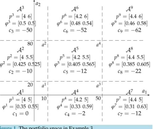
0 +cf=maxf∈Lcf .Example 3. Take into consideration the same two assets of Examples 1 and 2, with pay-off matrix,
2 8
6 4
=
X , and suppose that they are exchanged on the market as follows:
• X1 has unit price 4 for (short) sales or purchases up to 10 units, 4.2 for purchases up to 50 units and 4.4 beyond 50 units;
• X2 has unit price 5 up to 20 units, 5.5 up to 80 units and 6 beyond 80 units.
Such prices split the portfolio space into nine regions, identified by four vertices (see Figure 1). • 1 10
20
a =
, which yields the pay-off
1 180 140
a =
X and costs 4 10 5 20× + × =140;
• 2 10 80
a =
, which yields the pay-off
2 660 380
a =
X and costs 4 10× + ×5 20+5.5 60× =470 (recall the first 20 units of X2 are bought at the cheaper price 5, and only the 60 subsequent units are bought at the higher price 5.5;
• 3 50 20
a =
, which yields the pay-off
3 260 380
a =
X and costs 4 10× +4.2 40 5 20× + × =308;
• 4 50 80
a =
, which yields the pay-off
4 740 620
a =
X and costs 4 10× +4.2 40 5 20 5.5 60× + × + × =638. Inside each region, the unit prices i
p remain constant (shown in Figure 1 as well), and therefore the price
functional π is affine: we may write | i
i i i
f c
π = =ϕ + , i=1, 2,, 9. In greater detail: there have to be nine vectors 1 2 9 2
, , ,
ϕ ϕ ϕ ∈ and nine (non positive) constants
6
To prove the inequality, suppose that the cheapest (super) hedges for Y Z, ∈ are, respectively,
∑
nj=1βjXj and 1n j
j j=γ X
∑
, so that( ) 1
(
)
n j
j j
Y X
π =
∑
=π β and ( ) n1(
j)
j jZ X
π =
∑
=π γ . Let 0≤ ≤ϑ 1, and consider the portfolio n1(
(1 ))
jj j
j
W=
∑
= ϑβ + −ϑ γ X . Of course,(1 )
WϑY+ −ϑ Z; therefore, π ϑ( Y+ −(1 ϑ)Z)≤π( )W .
Since π( )W is defined as the cheapest (super)hedge of W, ( ) n1
(
(1 ) j)
j j
j
W X
π ≤
∑
=π ϑβ + −ϑ γ . On the other hand, the fact that all ofthe functions πXj (j=1, 2,,n) are convex w.r.t. α implies that
( )
(
)
(
)
( )(
)
( ) ( ) ( )1 1 1 1 1
n j n j j
j j j j
j=π ϑβ + −ϑ γ X ≤ j=ϑπ βX + −ϑ π γ X =ϑπ Y + −ϑ π Z
∑
∑
. By transitivity,( )
( Y 1 Z) ( ) (Y 1 ) ( )Z
π ϑ + −ϑ ≤ϑπ + −ϑ π , i.e. , π is convex.
236
Figure 1. The portfolio space in Example 3.
1, 2, , n
c c c ∈ such that, if X =Xa with a∈
(
j=1, 2,, 9)
, then π( )
X =ϕjX+cj. Every vector ϕj(
j=1, 2,, 9)
identifies a discount factor Bj and a risk-neutral probability Qj, and therefore this modelidentifies at least nine risk-neutral measures; however, as already pointed out, the risk-neutral measures turn out not to be as important as the properties of the price functional in order to investigate market efficiency.
Note that, if both X and X+H belong to the same region j, then π
(
X +H) ( )
−π X =ϕjH : it is then straightforward to realise that, for every j=1, 2,,n, the vector ϕjis easily determined by solving the usual linear system j j
p
ϕ X = . The constants cj, j=1, 2,,n, are calculated as the amount “saved” by buying the “first” units at a price smaller than pj
:
• In 1, the effective prices are the lowest ones: therefore, c1=0 (we could argue the same conclusion from
the fact that 0=π
( )
0 =ϕ1⋅ +0 c1);• In 2, the price of 2
X is 5.5, but the first 20 units are bought at the price 5=5.5−0.5, thus “saving”
20 0.5× =10: therefore, c2= −10 (as a double check, consider for instance that the portfolio 2 5
20
a= ∈
yields the pay-off 410
230
a=
X and costs 5 4× +20 5× +
(
50−20)
×5.5=285, and 2 2 410 285230 c
ϕ
= ⋅ +
pre-
cisely yields c2= −10);
• In 3, the price of X2 is 6, but the first 20 units are bought at 6− =5 1 less and the subsequent
(80−20=) 60 at 6−5.5=0.5 less, for a total “saving” of 20 1 60 0.5× + × =40: therefore, c3= −50 (note
that such a saving can also be calculated as the one achieved in the “previous” region 2, i.e., 20 0.5× =10,
plus the additional saving of 0.5 on all of the first 80 units: 20 0.5 80 0.5× + × =50); • In 4, the price of
1
X is 4.2, but the first 10 units are bought at 4.2− =4 0.2 less, thus “saving”
10 0.2× =2: therefore, c4= −2;
• In 5, both the first 10 units of
1
X and the first 20 units of X2
are bought at a lower price: the savings of 2 and 4 add up, and therefore c5 =c2+c4 = −12;
• In 6, the savings of 3 and 4 add up, and therefore c6 =c3+c4= −52;
• In 7, the first 10 units of
1
X cost 4.4− =4 0.4 less than the “full” price, and the subsequent (50 10− =) 40 cost 4.4−4.2=0.2 less: the total saving is 10 0.4× +40 0.4× =12: therefore, c7 = −12;
• In 8, the savings of 2 and 7 add up, and therefore c8=c2+c7= −22;
• Finally, c9=c3+c7 = −62.
Now, the price of every pay-off X∈2 can be calculated as
( )
max 1,2, ,9j
j j
X X c
π = = ϕ + . For instance, for 800
1200
X =
237
(the maximum price is emphasised). Note that, indeed, X is yielded by the portfolio 160 8
60
a= ∈
, and the
price of a is 10 4× +40 4.2 110 4.4× + × +20 5× +40 5.5× =1012.
As already mentioned, the price functional π is convex. We want nevertheless to strike out that, generally speaking, it is neither sub- nor superadditive: for instance, consider again the pay-off 800
1200
X =
. It is possible
to check that 800 350 0
π =
and
0
744 1200
π =
, and therefore
800 800 0
1012 1094
1200 0 1200
π = < =π +π
. On the other hand, it is also
400
495 600
π =
, and
therefore 800 1012 990 400 400
1200 600 600
π = > =π +π
. We want to point out that this second inequality
does not correspond to a convenient super-hedging: indeed, it is not possible to buy simultaneously two portfo- lios yielding the claim 400
600
because, when doubling the position, the unit prices of the traded assets increase.
It is still possible to show that, if π does not take infinite values, the set Φ =L:
{
ϕf :f ∈L}
is compact and convex. Mathematically speaking, the set ΦL is the union of the sub differentials ofπ
at all points X∈;note that, if π is sublinear, then Φ =L L.
In perfect analogy to what happens for sublinear functionals, π is increasing if and only if every ϕ ∈ΦL is
positive. The natural technique of pricing any pay-off Z (either belonging to or not) by super-hedging, as seen in Section 1.3, can still be applied, even in the case when π allows for convenient super-hedgings, and it can be shown that the cheapest super-hedging price π is a convex functional if the “original” π is. Further-more, the set ΦL corresponding to the set L identified by π turns out to be precisely the set
(
ΦL)
+ ={
ϕ∈ ΦL:ϕ0}
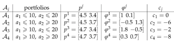
.Example 4. On Ω =
{
ω ω1, 2}
consider the two assets: • 1 45
X =
, at the unit price of 4.5, which increases at 4.7 for purchases of more than 10 units;
• 2 3 4
X =
, traded at 3.4 per unit, which increases at 3.7 for purchases of more than 20 units.
This way, 4 3
5 4
=
X . The prices split the portfolio space into four regions 1, 2, 3, 4, corresponding
to the four “quadrants” identified by the portfolio 10
20
a=
(see Table 1); note that the portfolio a yields the
pay-off 100
130
238
Table 1. The four regions of the portfolio space in Example 4.
previous Example 3, are also shown.
There are positive vectors in ΦL (such as 1
ϕ , for instance); yet, the negative components of ϕ2 and ϕ3
indicate the possibility of a convenient super-hedging. It is quite clear that such possibilities apply to all of the portfolios belonging to the regions 2 and 3.
Consider, for instance, the portfolio a2 = −
[
5 30]
∈2, whose pay-off is2 70 95
a =
X and whose price is
[
]
705 4.5 20 3.4 10 3.7 82.5 0.5 1.3 6 95
− × + × + × = = − ⋅ −
. It is immediate to check that the pay-off
2 70 95
a =
X
can be super-hedged by means of the portfolio 2
(
)
1 2 320
a = ∈
, whose pay-off is 72
95
and whose price
is 3 4.5× +20 3.4× =81.5<82.5: a convenient super-hedging is found, and the cheapest super-hedging price functional π will be such that 110 81.5
145
π ≤
(indeed, it can be shown that the equality holds).
Analogously, the portfolio 3
3 25 10
a = ∈
yields the pay-off
3 130 165
a =
X at the price
[
]
13010 4.5 15 4.7 10 3.4 149.5 1.8 0.5 2 165
× + × + × = = − × −
, but a convenient super-hedging is given by
(
)
3 4 3
17.5
20
a = ∈
, whose pay-off is 130
167.5
and whose price is 10 4.5× +7.5 4.7× +20 3.4× =148.25.
Therefore, 130 148.25 165
π ≤
(and, as before, the equality holds, indeed).
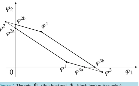
It is possible to prove7 that the “adjusted” functional π, calculated after exploiting all of the convenient su-per-hedgings, is calculated as the maximum of six affine functionals as shown in Table 2. Notably enough, the convex set Φ identified by the six vectors ϕ ϕ 1, 2a,,ϕ4 exactly amounts to the subset of the positive vectors contained in the “original” set Φ (see Figure 2). Note also that not all of the vectors ϕj, j=1, 2, 3, 4, induce risk neutral measures, because some of them have negative components; however, each of the six “vertices” of the “restricted” set Φ can again be seen as the product of a risk neutral measure and a discount factor (for in-stance, ϕ2b corresponds to the degenerate probability Q2b such that Q2b
(
{ }
ω2)
=1 and to the discount fac-7We confine ourselves to a few hints, in order to help a reader possibly interested in finding a method into this madness. In the region
2 ,
the “marginal” pay-off 1 0
(yielded by the “marginal” portfolio
4 5
−
) has a negative cost (indeed, 4 4.5× + − ×( )5 3.7= −0.5): therefore
the idea is to add to any portfolio
2 1 2 2 2 2 a a a = ∈
a multiple of
4 5
−
until “hitting” the boundary with another region. If
( 2 ) ( 2 )
2 1
4 a −20 ≤ −5 a −10 , such a region turns out to be 1, and the affine pricing functional used to price the pay-off becomes 2a
2a
c ϕ − ;
in the opposite case when ( 2 ) ( 2 )
2 1
4 a −20 ≥5 a −10 , the region hit is 4, and the “adjusted” pricing functional is 2b
2b
c
ϕ − . Analogous
considerations apply to the region 3, where the “marginal arbitrage” is the pay-off
0 1
, (yielded by the marginal portfolio
3 4 − ),
239
Figure 2. The sets Φ (thin line) and Φ (thick line) in Example 4.
Table 2. The four regions of the portfolio space in Example 4 after taking advantage of the convenient super-hedging opportunities.
tor B2b=0.925). Nevertheless, we remark that such elements are not as important as the ϕs themselves to
in-vestigate market efficiency.
When it comes to positivity, things get a little more complicated: indeed, the fact that Φ contains no posi-tive functionals at all is still sufficient, but no longer necessary, in order to allow for arbitrages. Consider the following (and quite minimal) example.
Example 5. Again on Ω =
{
ω ω1, 2}
, suppose that the asset1 1 0
X =
is sold at the unit price 0.4 regardless
of the amount, and that 2 0 1
X =
is sold at unit price −0.1 up to 5 units, and 0.5 for more than 5 units. The
portfolio space is trivially split into two regions (and in each of them, since 1 0
0 1
=
X , it is trivially
j j
p
[image:13.595.174.450.302.493.2]240
It is clear that arbitrages are possible, because buying 0
k
with k≥0 has a negative price for every
6
k< . Nevertheless, the set Φ contains the positive vector ϕ2 =
[
0.4 0.5]
.It is still possible to define the cheapest super-hedging price functional π: it turns out that it simply amounts to replace, in the region 1,
1
ϕ and c1 with
[
]
10.4 0
ϕ = and c1= −3. As a consequence, it is no longer
( )
0 0π = : indeed, π
( )
0 = −3, which precisely indicates the possibility to get a free gain of 3 without risk. It is also worth pointing out that such an arbitrage is just “local” in the spirit of Castagnoli et al. (2011), in the sense that there is an upper bound to the gains that can be obtained by means of arbitrages.The point is that, as already mentioned, an arbitrage is nothing but a convenient super-hedging of the null vector. In the sublinear case, positive homogeneity ensures that such a convenient super-hedging (meaning both its positive pay-off and its negative price) can be multiplied by an arbitrary positive constant and still remain an arbitrage: this way, if arbitrages are possible, the region of the arbitrage portfolios is always unbounded. In the “granular” convex case, instead, positive homogeneity no longer holds, and therefore arbitrages may be confined to a bounded region, as it happens in Example 5.
As a matter of fact, it is possible to show that a linear functional ϕ ∈Φ matters in determining whether π allows for arbitrages or not only if ϕ is relative to a “region” of the portfolio space that contains the null pay-off: we call Φ0 such a subset of Φ
8
. In other terms, while Φ is the union of all subdifferentials of π, we are here only interested in the subdifferential Φ0 of π at the origin. Briefly, a convex functional π is
positive if and only if there exists a positive ϕ ∈ Φ0.
For sublinear functionals, it can be proven that the subdifferential at each point is by necessity a subset of the subdifferential at 0, or, in other words that Φ = Φ0. This, besides the “unbounded” nature of arbitrages in
sub-linear markets, provides a further argument in favour of the fact that, unlike what happens for convex markets, in sublinear markets absence of arbitrages and absence of convenient super-hedgings are properties of the same set L.
The results of this section can be summarized and formalized in the following
Theorem 1. Let be a linear space of financial assets, and π:→ be a convex pricing functional such that π
( )
0 =0. Define L:={
f :→: f affine, f π}
and, for every f ∈L, call cf := f( )
0 and( )
:( )
f f cf
ϕ ⋅ = ⋅ − , so that f
( )
⋅ =ϕf( )
⋅ +cf. Let Φ =:{
ϕf : f∈L}
and Φ =0:{
ϕ:→:ϕlinear,ϕπ}
. Then:1. L is non-empty, closed and convex;
2. for every X∈, π
( )
X =maxf∈L f X( )
;3. for every f∈L, cf ≤0 and ϕf is linear; furthermore, there exists f∈L such that cf =0;
4. Φ and Φ0 are non-empty, closed and convex, and Φ =0 LΦ;
5. π is increasing if and only if every ϕ ∈ Φf is positive; 6. π is positive if and only if there exists a positive ϕ ∈ Φ0.
3. Increasing Average Prices
The Star-Shaped Case
Suppose that X∈ is such that the supply and demand function α→π α
(
X)
is convex. If, as it is nat-ural to suppose, π( )
0 =0, then it turns out that( )
( )
( )
( )
if 0 1, if 1
X X
X X
π α απ α π α απ α
≤ ≤ ≤
≥ ≥ (3)
the first inequality comes from the convexity property, because (being 0≤ ≤α 1) it is
8In the case when π( )0 =0,
0
Φ can also be defined as the subset of linear (not just affine) functionals of Φ or, equivalently, as the set
241
(
)
(
X 1 0)
( ) (
X 1) ( )
0π α + −α ≤απ + −α π ; it is furthermore possible to see that the two inequalities are equiv-alent to each other9.
A possible reason why inequalities (3) are sensible in ordinary markets can be seen as follows. Take
,
α β∈ such that 1≤ ≤α β, so that β α >1. The first of the two inequalities (3) above is equivalent to
(
X)
β X β(
X)
i.e., π β(
X)
π α(
X)
:π β π α π α
α α β α
= ⋅ ≥ ≥
in other words, the supply and demand function of an X∈ satisfies (3) if and only if the average unit price of X is increasing with respect to the traded amount. This is why we deem reasonable such a property: indeed, when aiming at purchasing some quantity of something, it is rational to buy it at the lowest possible overall price, which of course coincides with the lowest average unit price.
Suppose, for instance, that three agents sell the same asset X on the market. The first one sells it at 4 per unit, but can only provide up to 30 units. The second one sells it at 5 per unit (for any amount). The third one sells it at 4.5 per unit, but only for a minimum order of 50 units. It is clear that the best price that can be obtained to buy
0
α> units of X are:
(
)
4 30
5 30 30 60
4.5 60
X
α α
π α α α
α α
≤
= − < <
≥
for instance, to buy 50 units of X, the unit price of 4.5 may be obtained, but it is less expensive to buy 30 units from the first agent and 20 from the second, at a total price of 30 4× +20 5× =220 instead of 50 4.5× =225. Note that the average price obtained with the “separate” purchase is 220 50=4.4<4.5.
We shall call star-shaped a supply and demand function α→π α
(
X)
that satisfies inequalities (3) and, in general, any function f : →, with any real linear space, that does the same. Note the difference with “granular” pricing functionals, which feature an increasing marginal price with respect to the traded amount: of course every convex function is star-shaped as well, but the converse need not be true.Example 6. The function f :→ defined as
( )
0.3 102 1 10
x x
f x
x x
≤
= − >
is star shaped, because ( f
( )
0 =0 and) its “average value” f x( )
x is increasing. Nevertheless, f is notcon-vex (and not even continuous).
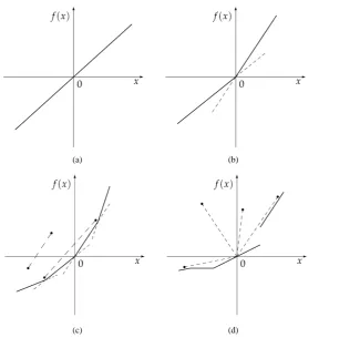
A geometrical interpretation of the star-shaped property is easily deduced from the monotonicity of average prices. Recall that, given any real linear space , a function f : → is convex if and only if, whenever two points
1 2
1 2
,
X X
y y
are given “above” the “graph” of f, i.e., such that
( )
j j
f X ≤ y
(
j=1, 2)
, then theentire segment adjoining
1
1
X y
and 2
2
X y
remains “above” the graph of f (which translates into
(
)
(
1 2)
(
)
1 2
1 1
f ϑX + −ϑ X ≤ϑy + −ϑy for every ϑ∈
[ ]
0,1 ). The property that average prices are increasing for star-shaped functions translates into the fact that whenever Xy
is given “above” the “graph” of f, i.e., such
that f
( )
X ≤y, then the entire segment adjoining 00
and
X y
remains “above” the graph of f (which
translates into f
(
ϑX)
≤ϑy for every ϑ∈[ ]
0,1 ). In Figure 3 the typical appearance of the four functions examined in this paper is depicted for functions f :→.9Define, indeed β 1
α
= and Y=αX: it is clear that 0≤ ≤α 1 (respectively, α>1) if and only if β>1 (respectively, 0≤ ≤β 1) and