Explaining the gaps in labour
productivity for some developed
countries
Razzak, Weshah
2006
Online at
https://mpra.ub.uni-muenchen.de/53/
in some developed countries
W A Razzak†
Department of Labour 56 The Terrace
Wellington New Zealand
Revised May 2006
Abstract:
Modern economic theories explain differences in productivity and economic growth across countries by differences in political and economic institutions, and differences in culture, geographical location, policies, and laws. The success of any of these theories in explaining the gap in productivity between any two countries depends on the countries in the sample. We argue in this paper that differences in the above variables might explain gaps in economic performance between developed and developing countries, but are too small to explain the productivity gaps between developed countries. We test this hypothesis for two pairs of developed neighbouring countries: New Zealand and Australia and Canada and the United States, hence New Zealand – Australia and Canada – United States. In this paper, more than eighty percent of labour productivity gaps between New Zealand and Australia and Canada and the United States are explained by endogenous technology shocks (TFP) and capital intensities.
Keywords: Labour Productivity, TFP, Real exchange rate JEL: O57, C13, C32
Productivity gaps between countries have always been an interesting problem for economists and policymakers. The literature is large and has several different strands. The neoclassical explanation of productivity gaps focuses
on exogenous Total Factor Productivity shocks (TFP), for example see,
Klenow and Rodriguez-Clare (1997), Hall and Jones (1999), and Parente and Prescott (2000). Recently, Cordoba and Ripoll (2005) provide a model of
endogenous TFP and show, analytically, that allowing for endogenous TFP
increases the role of input factors, i.e., capital and labour, in explaining the gap in income between countries.
In endogenous growth model(s) economic institutions are cited as
fundamental “causes” of cross-country differences in economic development because they influence economic outcomes by shaping economic incentives,
e.g., Acemoglu et al. (2004), Diamond (1997) and Myrdal (1968) (for a
literature review about the role of institutional differences, see for example, Nelson and Sampat, 2001).
Other strand of the literature related to the “New Economy” hypothesis focuses on the role of GPT, e.g., Helpman and Trajtenberg (1998) and Helpman (1999), and another focuses on the role of Information and
Communications Technology, ICT (e.g., Basu et al. 2003) on TFP. They try to
explain productivity gaps between the United States and the United Kingdom.i
In Helpman (1999), Lipsey et al. provides a discussion about the lagging pace
of General Purpose Technology (GPT) growth in Canada relative to that of the United States and suggests that it can explain Canada’s poor productivity performance relative to the United States. Harris (2001) argued that the Canadian real exchange rate depreciation can explain gaps in labour productivity and provides empirical evidence for the case of Canada and United States.
Furthermore, Sachs (2000) argues that economic geography is a crucial explanatory factor of growth gaps. There is a new literature, where cross-country growth and productivity gaps are explained by differences in the legal systems, i.e., common versus civil laws, via their effect on the financial
markets, see for example, Mahoney (2000), La Porta et al. (1998 and 1997)
and King and Levine (1993).
Culture (e.g., religion, language etc.) that generates a set of beliefs, which emphasise thrift and saving, for example, affect economic development via the effect on the accumulation of capital as in Weber (1930), and Greif (1994).
See Barro and McCleary (2003) and Tabellini (2005)for empirical evidence.
In this paper we argue that the above theories are more appropriate to explain the gap in productivity between developed and developing countries, but they cannot empirically explain a large portion of the productivity gap between developed countries.
To illustrate, think of New Zealand and Australia and Canada and the United States. Both New Zealand and Canada have poor productivity relative to their big neighbours Australia and the United States. We choose these two pairs of countries: New Zealand – Australia and Canada – United States because we could control for many of the variables mentioned above. These countries are highly developed; have similar cultures; language; and similar political and economic institutions. They are among the world highly prosperous Western democracies. According to OECD they have relatively highly educated labour forces and flexible product and labour markets.
New Zealand, Australia and Canada have similar monetary policy framework, i.e., price stability, independent central banks etc, and the United States has a very similar monetary policy in the sense that the Fed also cares about price stability and it is independent. About 85 percent of the banking system in New Zealand is owned by Australians. Capital moves freely between New Zealand – Australia and Canada – United States, and in New Zealand – Australia, labour also moves freely.
New Zealand – Australia and Canada – United states are neighbours so geographically speaking they are equally distant from the rest of the world. The laws in New Zealand and Australia are pretty similar or at least have a similar origin – i.e., common law. We conjecture that a similar argument applies to Canada and United States and differences in the laws cannot possibly account for the large and persistent gap in labour productivity.
Canada – United States’ differences in GPT investments might be big and
could explain some of the productivity gap. However, Tullett et al. (2002)
argue that New Zealand’s ICT intensity (expenditures as a percent of GDP) is among the highest in the world, and ahead of Australia so it is possible that ICT and GPT can explain productivity gaps in developed countries on a case
by a case basis.ii
Both New Zealand and Australia embarked on a wide reform process in the
mid 1980s so we chose a post-reform sample.iii The sample is from 1989q1 –
2003q4. The period before the reform (1984) is irrelevant for the objective of this paper, i.e., we want to explain the gap in labour productivity that has occurred despite similar economic reforms in both countries. For Canada – United States we choose the period 1985q1-2004q4 because Canada experienced a lower labour productivity than the US in the 1990s and that is what we want to explain.
to be the most comprehensive free trade agreement in the world. Canada and the United States signed a free trade agreement in 1989.
Section 2 provides stylised facts and outlines the problem. Section 3 discusses the model. Results of estimation are reported in sections 4. Conclusions are in section 5.
2. Stylized facts
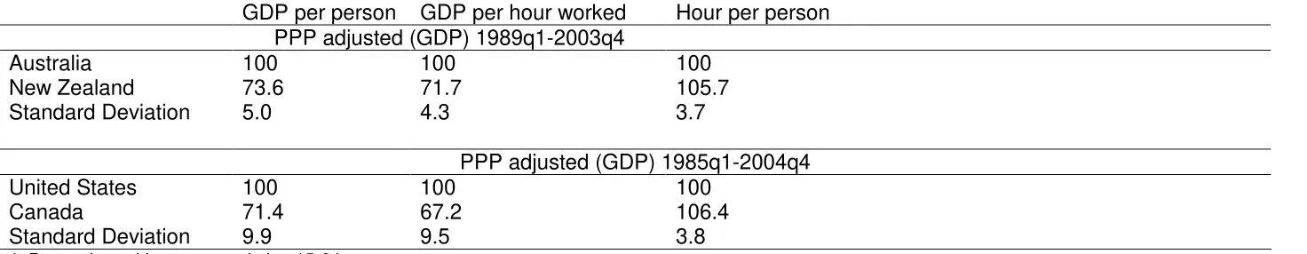
All the data are found in the data appendices. Table 1 reports the
PPP-adjusted data for New Zealand – Australia and Canada – United States.iv It
decomposes real GDP per person into real GDP per worked and
hour-worked per person (
t t
t t
t t
P H H
Y
P Y
ˆ .
ˆ = ), whereYtis real GDP,Htis hour-worked
andPˆtis working age population.
Table 1 shows that real GDP per person is lower in New Zealand compared with Australia (73 percent of Australia’s), thus, New Zealand is poorer. Real GDP per hour-worked is also lower in New Zealand (71 percent of Australia’s) so New Zealanders are less productive than the Australians. Although New Zealand’s productivity might have improved relative to its own past history (i.e., after the reform in 1984), its income remained low relative to Australia because Australia has been even more productive.
Similarly, Canada’s PPP-adjusted GDP per person is smaller than that of the US (71 percent of the United States’) and GDP per hour-worked is
substantially lower than that of the United States (67 percent of the United States’). Interestingly, both New Zealanders and Canadians work only slightly longer hours than their next doors’ neighbours over the two samples. Also, relative GDP per person and GDP per hour in the case of Canada – United States are more variable (i.e., larger standard deviations) than those of New Zealand – Australia.
There is a widespread belief among New Zealanders that the Australian’s productivity superiority is due to having a vast mining industry, which has a huge capital investments and hence, a higher marginal product of labour, e.g., Matheson and Oxley (2004). Table 2 reports the same decomposition of table 1 for New Zealand and Australia, except that GDP of the mining industry is removed from the Australian GDP. Clearly, removing the Australian mining industry makes only a small difference. Table 3 shows that mining is not an issue for the growth rate of the gap in GDP per hour-worked in New Zealand – Australia case. The mean and the standard deviation of the productivity gap (GDP per hour-worked) growth rate are identical.
3. The model
) , (
1 YtT = AtTΚ KtT HtT ,
) , (
2 YtN = AtNG KtN HtN ,
The superscriptsTandN denote tradables and nontradables respectively.
whereYtis real output,Ktis the stock of capital,Htis hour-worked, and
T t
A is a
technology shock to tradables, TFP and N
t
A is technology shocks to
nontradables. To keep things simple, it is assumed that there are no
intermediate inputs in production. Normalizing byHt:
) 1 , ( 3 T t T t T t T t T t H K A H Y Κ = ) 1 , ( 4 N t N t N t N t N t H K G A H Y =
Taking logs –lower-case:
T t T
t T
t a k h
h
y ) ( )
(
5 − = +κ −
N t N
t N
t a g k h
h
y ) ( )
(
6 − = + −
Summing (5) and (6) gives us:
t N
t T t
t a a F k h
h
y ) ( ) ( )
(
7 − = + + − ,
where(y−h)tand (k−h)tare the aggregates including both tradables and
nontradables. TFP in tradables and nontradables are left separated. Thus, the gap in GDP per hour-worked or the gap in labour productivity is a function of the TFP shocks in tradables and nontradables, and the gap in capital intensity.
The foreign country has the same functions, where f denotes foreign country.
f t f f N t f T t f
t a a F k h
h
y ) ( ) ( )
(
8 − = + + −
Subtracting (8) from (7) and letting double prime on the variables denote the gaps between the home and the foreign magnitudes. We arrive at:
t N
t T t
t a a F k h
h
y ) ( ) ( )
(
9 − ′′= ′′ + ′′ + ′′ − ′′
In this paper, TFP in tradables and nontradables are endogenous and depend on a variety of variables linearly. TFP in tradables at home, abroad and the gap are given by the linear functions:
T t t t t t T t
a =Γ(µ ,ψ ,ο ,α )+ε 10 Tf t f t f t f t f t f Tf t
a =Γ µ ψ ο α +ε
′ ( , , , )
T t t t t t T
t
a′′ =Γ ′′ µ′′ψ ′′ ο′′α′′ +ε′′
′′ ( , , , )
0 1
Whereµdenotes manufacturing;ψ denotes the stock of knowledge; ο
denotes openness; and α denotes aging. We explain the hypotheses
underlying the choice of these variables.v
Manufacturing:The relationship between manufacturing output and
productivity is known as the Verdoorn’s Law (1949). It says that there is a
strong statistical relationship between manufacturing output and labour
productivity and that causality runs from the former to the latter. This is usually interpreted as evidence of increasing returns to scale. Arrow (1964)
cited The Verdoorn’s Law and recently, McCombie et al (2002) provides a
collection of articles on this relationship. See Libanio’s book review in the Economic Journal (2005). This is also consistent with Delong and Summers (1991), where they document a robust relationship between productivity growth and changes in the stock of capital machinery and equipment in the United States.
Manufacturing and industrialisation are usually perceived as processes associated with industries like steel, cement, cars…etc with their negative environmental and social consequences. However, there is a lot of
productivity gains associated with manufacturing, whether it is old or new. Today, most industrial nations think of new and green manufacturing, where production involves lots of R&D and human capitals in addition to capital and
labour intensities. The future is for this new type of manufacturing, which is
environmentally friendly, smart, and involves a lot of R&D and human capitals. Countries which seek growth and productivity gains are willing to leap and skip steps directly into new manufacturing. New Zealand, for example, have potentials to produce new goods and services along these lines, e.g., fuel from sheep manures (there are more than 40 million sheep in New Zealand); a new generation of healthy dairy products with medicinal properties; marine products; marine drugs and bio-technology; wine; movies and related fields
etc, which are new goods and services with potentially very large productivity
gains.
A variable that best proxy manufacturing is the stock of manufacturing. It is defined as the sum of stocks of materials and finished goods on the factory floor including work in progress. Goods and Services Taxes (G.S.T.) are excluded. A country that exports furniture, for example, would have timber, processed timber, and furniture in its stock of manufacturing while a country that exports timber will have nothing on its manufacturing floor.
Knowledge: The relationship between knowledge and productivity us well
understood in economics. For theoretical models see for example, Barro and Sala-i-Martin (1995), Grossman and Helpman (1991) and Aghion and Howitt (1992) for growth models that include R&D spillovers. Romer (1986) and
Lucas (1988), Mankiw et al. (1992) and Rangazas (2005) are examples,
for a survey of the literature at the micro-level. The stock of R&D isa widely used proxy for knowledge.
Openness: Economic theory is not ambiguous about the effect if trade on
economic growth. There is a positive relationship. At the micro-level, the hypothesis is that openness or increasing trade would expose local firms to foreign competition, which forces weak unproductive ones to exit and strong ones to expand and prosper. Also, openness brings with it foreign goods, which embodies foreign R&D technologies and there might be positive
spillovers into domestic production.vi There are measurement issues and
openness could be measured in a variety of ways. In this paper we use a common measure of openness: Total trade (sum of exports and imports) as a percentage of GDP is used as measure of openness.
Aging: It affects technical progress by affecting the relationship between
workers and technology, i.e., use, adoption and creation of new technologies along the growth and development process, where old jobs are destructed and new ones are created continuously. A commonly stated hypothesis that older workers resist changes and fight against new ideas and technologies
and thus adversely affect labour productivity growth, is tested.vii There are,
however, other hypotheses, where older workers might be more experienced, loyal etc and thus, have positive effect on productivity of the firm. The
literature stretches across various disciplines. The empirical evidence is mixed. In this paper we measure the aging gap as the gap between employed workers age 55+ to total labour force in the two countries.
There is another important aspect of the aging data in New Zealand. Davey (p.46, 2003) reports that 1/3 of the people aged over 50 have no qualifications and the educational achievement declines with age. In the past, the
proportion of workers with no formal qualification was quite substantial, 30 percent in 1985. However, this percentage has been falling over time. It is 18 percent in 2003. Unfortunately, similar data for Australia are not readily
available.viii
The variablesµt, f
t
µ ,ψt , f t ψ οt,
f t
ο ,αtand f t
α are assumed to follow a random
walk processes with drift. It is assumed that the foreign country has a similar model in specifications and parameters and only differs in the realization of the shocks. This implies that the two country’s growth rates can differ in the short-run and converge in the long run.
Similarly, N
t
a and Nf
t
a are assumed to be functions of productivity in the
services industries, and that these service productivity data are random walk with drift. It is further assumed that productivity in the service sector is
measured with error.ix Substituting back in (9) and assign some parameters,
we get:
t t t
t t
t t
t k h sr u
h
y− )′′= ( − )′′+[ 1 ′′−1 + 2 ′′−1 + 3 ′′−1 + 4 ′′−1]+ ′′−1+ ′′
(
11 β π µ π ψ π ο π α θ
In terms of growth rates,
t
t v
a′′=∆ ′′ ∆
12
and
t t sr t
t t
t t
t k h v v v v v u
h
y− ′′= ∆ − ′′+ ∆ ′′ + ∆ ′′ + ∆ ′′ + ∆ ′′ + ∆ ′′ +∆ ′′
∆( ) ( ) [ 1 , 2 , 3 , 4 , ] ,
13 β π µ π κ π ο π α θ
Thus, labour productivity gap is a function of (1) capital intensity gap (k−h)t′′,
where we expect β >0and (2) TFP shocks in tradables and nontradables at
home and abroad. The variables ∆vµ′′,t ∆vα′′,tare the shocks to the gap in
manufacturing stock, gap in knowledge, the gap in the degree of openness and the gap in aging of the labour force. The model predicts that TFP in tradables drives labour productivity, and that countries become richer mostly through improvements in productivity in tradables. The model predicts that all
coefficients to have positive signs, i.e.,π1 >0,π2 >0,π3 >0,π4 >?and θ >0.
The coefficient π4(the shock to aging) might have an ambiguous sign.
All data are plotted and fully defined in the appendix 1 and 2. In the appendix we examine the time series properties of data, i.e., test for unit root. We used a variety of time series tests for unit root with different specifications (see appendix for details). The hypothesis of unit root could not be rejected for the gaps in the levels, but easily rejected in the growth rates. We have no theory for cointegration. In other words, there is no a priori reason to expect the gap in labour productivity between two countries to be cointegrated with gaps in aging or openness etc.
Note that the plotted real exchange rate is the inverse of the real exchange rate used in the regressions later for illustrative purpose. In the plots, an increase in the real exchange rate denotes an appreciation. In the
regressions, an increase in the real exchange rate denotes depreciation. The data are PPP-Adjusted. We do not have adequate data for human capital stock and for this reason we drop it from estimation.
4. Estimation and results
4.1. New Zealand – Australia
We begin with estimating a single equation model in both the level and the
growth rate.x
Two estimators are used, OLS and GMM (Generalised Method of Moments).xi
data-generating process is unknown to fully trust FIML so GMM is the second best choice. The drawback for GMM is that there are no good instruments. For
instruments, lags of the regressors and a constant are used.xii
Visually examining the data in appendix 1 shows that productivity gap is highly correlated with the real exchange rates, the gap in capital stocks, the gap in manufacturing stocks and in R&D gaps. This is true in the levels and in growth rates. This is also true for the Canada-United States data.
Single-equation regressions are reported in table 4.xiii All the regressions
include lagged dependent variable. The gap in capital intensity is statistically significant and has a positive sign in all four regressions. The magnitude of coefficient is the same in three regressions; GMM in the level, GMM in the growth rate, and OLS in the growth rate. The coefficient is smaller in OLS level regression. A similar result is obtained for the gap in the manufacturing stock. For the gap in R&D, the parameter estimates are positive and highly significant in all regressions. The magnitudes vary slightly across estimators. These three variables seem to have most of the explanatory power.
The parameter estimate for openness is insignificant in all four regressions and in the level regressions the coefficients have negative signs. But one would not have guessed this from visual inspection of the data in figures a21 and a22. These results are not surprising since the empirical literature provides no or very little evidence for association between openness
measured by export plus imports as a percentage of GDP and GDP growth in cross-sectional growth regressions.
The majority of the evidence in the literature is cross-section. Rodriguez and Rodrik (2001) and Rodriguez (2006) examine the international evidence carefully and show that measurements of openness and methods of estimation are the main reasons for obtaining different results in growth regressions. They argue strongly that no significant statistical relationship is found between openness and growth in cross-sectional growth regressions. We will further discuss this issue in the next section and show that this may not be necessarily true in general.
F igure 1: A ge pro f ile o f t he la bo ur f o rc e ( a v e ra ge o f 19 8 6 a nd 2 0 0 3 )
0 1 2 3 4 5 6 7
55-59 60-64 65+
New Zealand Australia
% o f labo ur fo rce
Services productivity, which is a proxy for productivity in nontradables is negative and only significant in the growth rate regressions. This coefficient has the wrong sign. It is either because the equation is misspecified in this variable or the measurement of the variable caused the sign reversal. We suspect that measurement is an issue.
The residuals are thoroughly tested for serial correlation and normality using a battery of tests. We found no evidence of serial correlation and they appear
to be normal.xiv The goodness of fit is not very high in GMM regressions, but
80 percent of the variations in the productivity gap are explained by OLS and FIML. Next, we will provide more evidence by considering the joint effect of effect of TFP shocks on the real exchange rate and labour productivity.
4.2. Productivity and the real exchange rate
A few Canadian papers associate the gap in productivity between Canada and the United States with the real depreciation of the Canadian dollar. Harris (2001) argues that causality runs from the real exchange rate to productivity. He explains why Canada’s productivity is lower than that of the United States by estimating a productivity convergence equation, where changes in
productivity in industry i in country cat time t depends on country and
industry fixed effects and a set of explanatory variables such as R&D investments, human capital intensity, openness, and trade specialisation in addition to the real exchange rate.
There are a few hypotheses, where real depreciations increase the cost of imported capital equipments and R&D, affect exports then output, or induce firms to substitute investments in R&D with output-expanding activities. He finds evidence that real depreciation affects productivity growth. Sustained real deprecations have negative effects for the long term productivity growth.
The real exchange rate (the relative price of nontradables) and relative productivity are related via the HBS effect. Given the production functions in tradables and nontradables the representative firm maximises its
intertemporal profit, which is given by:
∫
∞ − − − + 0 ) ) , ( ) , ( [14 Max YtT KtT HtT PYtN KtN HtN WtHt It e Rtdt
subject to:
t t
t I K
K = −δ
∆ +1
15
The variables are the same that we defined earlier,Ptis the relative price of
non-tradables in terms of tradables;Wt is the wage rate, which equalises
across tradables and nontradables overtime; the aggregate labour supply is
the sum of T
t
H and N
t
H ;Itis investment;Rtis the foreign real interest rate
andδ is the depreciation rate of capital. In equilibrium, we get the typical
FOC: r N t N t t T t T
t K P Y K R
Y ∂ = ∂ =
∂ / ( / ) 16 t T t T t N t N t
t Y H Y H W
P(∂ /∂ )=∂ /∂ =
17
1 18 λ =
Thus, the relative price of nontradables is equal to the ratio of the marginal product of labour in tradables and nontradables, i.e., relative productivity:
) / /( ) / (
19 Pt = ∂YtT ∂HtT ∂YtN ∂HtN
Given that the log real exchange (qt =st + pt* − pt) is also the relative price of
nontradables, the general price levels *
t
p andptare linear combinations of
tradables and nontradables prices, and Purchasing Power Parity (PPP) holds, the HBS is typically expressed as follows:
t N t T t
t a a
q =τ( ′′ − ′′ )+ξ 20
Andτ <0, which implies that the home country will experience real
appreciation, i.e., a rise in its relative price of nontradables, if its technical progress (TFP) in tradables exceeds its technical progress (TFP) in nontradables.
We substitute for the technology shocks gaps in the real exchange rate
equation above and maintain the assumption that nontradables productivity is approximated by service sector productivity, which is observed with error as described earlier; we arrive at:
t t t
t t
t sr
q=τ[π µ′′− +π ψ ′′− +π ο′′− +π α′′− −θ −′′ ]+ξ
The relative price of nontradable is driven by the same TFP shocks that drive
labour productivity. Given the way we measure the real exchange rate,τ is
expected to have a negative sign, i.e., an increase in TFP shocks in the tradable sector appreciates the real exchange rate.
The real depreciation rate is:
t t sr t
t t
t
t v v v v v
q =τ π ∆ µ′′ +π ∆ κ′′ +π ∆ ο′′ +π ∆ α′′ −θ∆ ′′ +∆ξ
∆ [ ]
22 1 , 2 , 3 , 4 , ,
The cross-equation restrictions in equations (13) and (22) suggest that the
coefficientsπ1toπ4are the same with opposite signs.
The empirical literature and evidence for HBS effect is mixed.xv Rogoff (1992)
noted that most of the evidence in favour of the HBS effect was found in countries that have closed capital markets. None of the countries in our sample has a closed capital market. Effects of government expenditures, oil prices and the term of trade as additional explanatory variables in the Harrod – Balassa – Samuelson equation are also mixed.
New Zealand – Australia: We start testing the New Zealand – Australia data.
We estimate unrestricted two-equation system. We are more interested in the growth regressions than the levels because of the time series property of the data. But we also estimated the model in levels. We don’t report the results to
save space, but they are available upon request.xvi
We follow the same estimation strategy. We estimate an unrestricted system in growth rates. We test the restriction that the four coefficients of the shocks to the stock of manufacturing, shocks to R&D stock, openness shocks and ageing shocks are the same in the productivity gap equation and the real depreciation equation. The coefficients are expected to have same magnitudes, but differ in the sign. Results are reported in table 5.
In the GMM regression, the restriction that the R&D shock has the same magnitude in the productivity gap and the real exchange rate equations is rejected. The P value of the Wald test statistic is 0.00. Also, the restriction that the coefficients of the services productivity in the two equations are equal is rejected. In the FIML regression, the restriction that the coefficient of the aging shock is equal in both equations is rejected. The P value of the Wald test statistic is 0.0016. All other restrictions seem to hold.
In table 6 the estimation results of the restricted system in growth rates are reported. We imposed the restrictions that passed the tests in table 5 on the system. The capital intensity gap has significant, positive and robust
coefficients across estimators. The magnitudes of the coefficients are 0.25 and 0.19 for GMM and FIML respectively.
in the GMM regression. In the productivity gap equation the coefficient is 0.27, positive and significant. In the real exchange rate equation it is
insignificant. In FIML, the restriction is imposed and the coefficient estimate is 0.25 and significant.
Openness shocks are insignificant. We got the same result in the single-equation regression earlier. Trade gaps measuring the degree of openness have no direct impact on labour productivity. What matters for productivity is perhaps the domestic value added of exports per unit of output. Data are not readily available and this might be a subject for future research.
Aging has a significant negative effect on labour productivity with a coefficient 0.14 in GMM. In FIML, the restriction that aging affects both labour
productivity and the real depreciation rate is not imposed. The
coefficientπ14has a negative sign, but insignificant. However,π24is large 0.35
and positive, which along withτ being negative implies that aging appreciate
the real exchange rate. We don’t have an obvious explanation to this result.
In GMM, we don’t impose any restrictions on productivity in nontradables so
we have two coefficientsθ11andθ21. Nontradables productivity seems to have
a significant negative impact on labour productivity and no impact on the real
exchange rate. The size ofθ11is 0.60, which is much larger than all other
coefficients in the model. In FIML, the restriction that the two coefficients are the same is imposed. It turned out that the sign is negative, but the coefficient
is insignificant.xvii
In the real depreciation equation, the coefficientτ is negative as expected. The
coefficient estimate is also highly significant in both the GMM and FIML regressions. The negative sign along with the positive signs of the
coefficients of∆vµ′′,t and∆vψ′′,t implies that an increase in the shocks to
manufacturing stocks and R&D stocks appreciate the real exchange rate, which is difficult to explain. Aging appreciates the real exchange rate, which is not intuitive. An increase in the nontradables shock proxied by services has no effect on the real exchange rate and this is consistent with international evidence and most likely due to measurement problems. The real
depreciation rate is highly persistent.
Canada – United States: Again, we estimated unrestricted two-equation
system in the levels for Canada – United States. We don’t report the results
to save space, but we tested the restriction on the coefficients.xviii
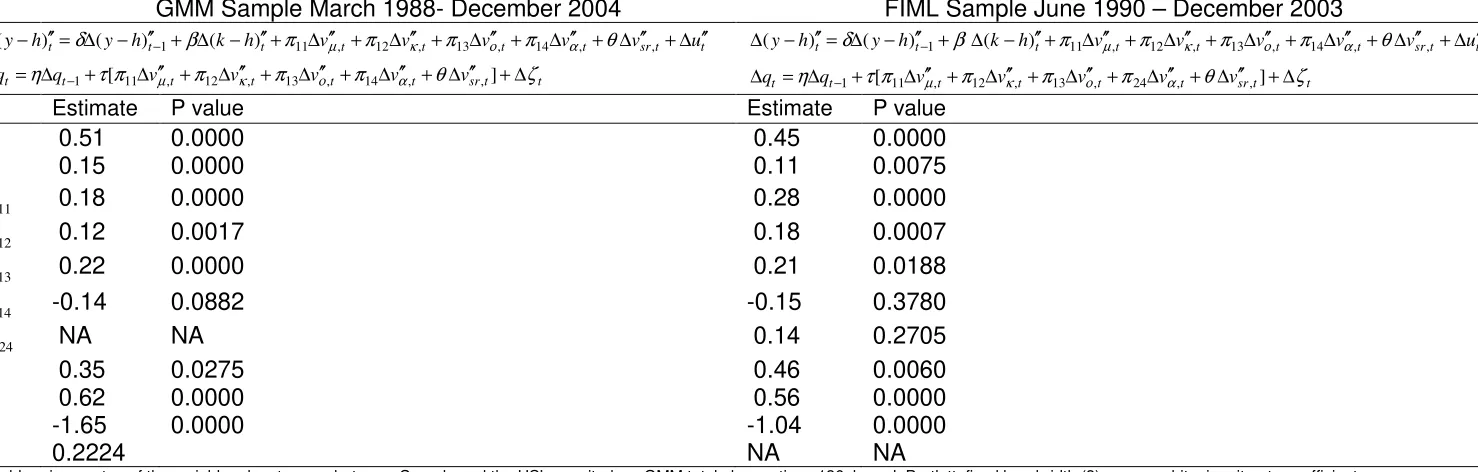
We then impose these restrictions and estimate the system. Results are in table 8. Labour productivity is more persistent, with coefficient of the lagged dependent variable ranging between 0.51 and 0.45 compared with 0.06 in New Zealand –Australia data. In GMM, all variables are statistically significant and have the predicted signs. The capital intensity gap has a coefficient estimate of 0.15 and 0.11 in GMM and FIML respectively. The sizes of these coefficients are smaller than the ones in the New Zealand – Australia case, 0.27 and 0.19 respectively.
Shocks to the stock of manufacturing and the stock of R&D have similar magnitudes to those in the New Zealand –Australia data. However, unlike the case in the New Zealand – Australia case, openness shocks are positive and significant with large coefficients in GMM and FIML. Ageing shocks are negative and significant in GMM. In FIML, aging enters with two separate coefficients in the productivity gap and the real depreciation equations. It is negative, but insignificant in the productivity gap equation. It is insignificant in the real depreciation equation. The real depreciation rate is also highly
persistent. The Canada – United States data seem to fit the model pretty well.
Services productivity has the expected positive sign and significant in both GMM and FIML. It means it positively affects labour productivity and
becauseτ is negative it means that it appreciate the real exchange rate, which
is inconsistent with the Harrod – Balassa – Samuelson theory. Again, these results are consistent with international evidence.
We thoroughly test the residuals of each equation using a variety of tests for whiteness such as the Fisher-Kappa and the Bartlett – Kolomogrove – Smirnov tests in the frequency domain even though the Newey-West
procedure is used to estimate a consistent variance-covariance matrix, thus
serial correlation and heteroscedasticity-robust estimates. The 2
R statistics of
the individual equations are pretty high ranging from about 0.76 to 0.90. To assess the goodness of fit further stochastic simulation is used to assess the goodness of fit for both the New Zealand – Australia and Canada-United States systems. The two-equation system is solved forward and backward over the sample periods. A Monte Carlo simulation solved the model 10,000 times using random shocks and generated distributions for the two
endogenous variables in the model. The method is Gauss-Seidel. Initial starting values are last period’s solutions, not actual. At each observation of a stochastic simulation, a set of independent random draws are taken from the standard distribution. These numbers are multiplied by Cholesky factor of the co-variance matrix. Confidence bounds are sample quantile estimates of the underlying distribution computed not from the entire sample, but using Jain and Chlamtac (1985) to conserve on memory use and with 10,000 repetitions. The tails of the distributions are pretty well estimated.
from FIML is in a thick grey colour. I also plot the average of the upper and lower confidence bands from GMM and FIML. These are plotted in the same colour, but the lines are dotted. In the case of New Zealand – Australia, TPF shocks – condition on capital per hour – explain about 80 percent of labour productivity growth gaps and 60 percent of the real depreciation rate. FIML fits the data better; TFP explains about 80 percent of labour productivity growth gaps and more than 80 percent of the real depreciation rate. In the Canada – United States data, more than 80 percent and close to 90 percent of data are explained by TFP shocks.
2: New Zealand-Australia Mean Stochastic Baseline Labour Productivity & Confidence Bounds
-0.2 -0.1 0 0.1 0.2
199219931994199519961997199819992000200120022003
d(y-h)" GMM Mean FIML Mean
upper low er
3: New Zealand-Australia Mean Stochastic Baseline the Real Depreciation Rate & Confidence Bounds
-0.3 -0.2 -0.1 0 0.1 0.2
199219931994199519961997199819992000200120022003
dq
GMM Mean FIML Mean upper
low er
4: Canada-US Mean Stochastic Baseline Sim ulation for Labour Productivity and Confidence Bounds
-0.2 -0.1 0 0.1 0.2 0.3
198719881989199019911992199319941919959619971998199920002001200220032004
(y-h)" GMM Mean
5: Canada - US Mean Stochastic Baseline Sim ulation for Depreciation Rate and Confidence Bounds
-0.3 -0.2 -0.10 0.1 0.2
198719881989199019911992199319941995199619971998199920002001200220032004
dq GMM Mean
upper low er FIML Mean
5. Conclusions
There are many different economic theories to explain economic growth and productivity gaps across countries. While many economists showed that exogenous TFP shocks can explain differences in labour productivity others cited institutional differences as the main variables to explain cross-country differences. Still others suggested differences in laws and cultures as the main explanatory variables for cross-country persistent gaps in productivity. Geography is also cited as a crucial variable. Others attempted to explain differences in productivity between countries by differences in GPT (General Purpose Technology) and ICT (Information and Communication Technology) gaps for the cases of the United Kingdom – United States and Canada – United States. Finally, the real exchange rate was cited as the variable that explains the Canadian – United States productivity differences.
There is a web of specifications and estimation issues in these literatures. The definition and measurement of productivity varies from one paper to another. Even when the relationship between productivity and the real exchange rate is the main issue (i.e., Harrod –Balassa – Samuelson) it is not clear whether productivity is labour productivity or TFP.
While it is highly conceivable that differences in institutions, culture, laws, and geography can explain productivity differentials between developed and developing countries they are too small to explain productivity differentials between two neighbouring fully developed industrial countries like New Zealand and Australia and Canada and the United States. There must be a large gap in ICT and GPT between the United States and all other developed Western industrial countries in the 1990’s, but Prescott (1997) argues
convincingly that the home country need not be the centre of R&D in the world nor need to have massive R&D infrastructures to support growth in
productivity because openness ensures that the small country can adopt certain foreign technologies. New Zealand, for example, is on the top of the OECD countries in the expenditures and use of ICT and it is hard to argue that there are large differences between New Zealand and Australia’s institutions, culture, laws, distance from the rest of the world to explain the persistent gap in productivity.
hour-worked is a function of capital intensity (capital per hour-worked or capital per unit of output) and technical progress, TFP. The real exchange rate is a function of TFP differential in tradables at home and abroad and TFP differential in nontradables at home and abroad. In this model TFP is
endogenous, and modelled as a linear function of the stock of manufacturing, the stock of knowledge proxied by R&D stock, the degree of openness
measured as the sum of imports and exports as a percent of GDP and
ageing, measured by of employed workers aged 55 and more as a percent of the labour force.
The relationship between manufacturing and productivity goes back to the Verdoorn’s Law cited in Arraw (1964) classic paper on learning-by-doing and consistent with Delong and Summers (1991) – increasing returns to scale. R&D stocks is a familiar proxy for knowledge in economic literature, and openness is said to enhance productivity because competition with foreign firms and imported products that embody foreign R&D forces less productive firms either to exit or to work hard to compete. Older labour force is less adoptive to new technologies and hence less productive. These variables are assumed to follow random walk with drifts. It is also assumed that the foreign country has a similar model in specifications and parameters and only differs in the realization of the shocks.
Because the real depreciation rate – the relative price of nontradables – is also a function of the same variables, TFP shocks drive both, the growth rate of labour productivity gap and the real exchange depreciation rate with
appropriate and testable cross-equation restrictions.
The two-equation system model is estimated for New Zealand – Australia (1989q1-2003q4) and Canada – United States (1985q1-2004q4). The model fits the data well, especially in the Canada – United State case, where most of the predictions of the model seem to hold. Stochastic simulation indicates that it explains between 80-90 percent of the growth rate gaps in labour productivity and the depreciation rates in the four countries. The cross-equation restrictions implied by the model hold well. Given that TFP shocks can explain 80-90 percent of the real exchange rate depreciation rate, no attempt was made to test the effect of demand side variables on the real exchange depreciation rate.
We conclude that (1) gaps in growth rates of labour productivity measured in terms of real GDP per hour-worked and the real exchange depreciation rate – are driven by the same random TFP shocks and ought to be modelled and estimated jointly as a system with appropriate and testable cross-equation restrictions. Hence, there is evidence for the HBS effect; (2) TFP is
endogenous and it depends on many variables important among them are the gap in the stock of manufacturing, which we proxy by the stocks of
manufacturing and knowledge, which is proxied by the stock of R&D, the degree of openness measured as the share of imports plus exports in GDP and ageing, which we proxy by employed workers 55 and over as a
References
Acemoglu, D. S. Johnson and J. Robinson, “Institutions as the Fundamental Cause of Long-Run Growth,” A paper prepared for the Handbook of Economic Growth, Philippe Aghion and Steve Durlauf (eds.,), 2004.
Aghion, P. and P. Howitt, “A Model of Growth Through Creative Destruction,” Econometrica 60, 2, 323-351, 1992.
Arin, K. P. and F. Koray, “Fiscal Policy and Economic Activity: US Evidence,”
Working Paper presented at15th New Zealand Econometric Study Group,
Auckland University of Technology, 2005.
Balassa, B., “The Purchasing Power Parity Doctrine: A Reappraisal, Journal of Political Economy 72, 584-596, 1964.
Barro, R. and X. Sala-i-Martin, Economic Growth, MIT Press, 1995.
Barro, R. and R. McCleary, “Religion and Economic Growth,” National Bureau of Economic Research Working Paper No. 9628, 2003.
Basu, S., J. G. Fernald, N. Oulton and S. Srinivasan, “The Case of the Missing Productivity Growth,” NBER conference April 2003.
Chinn, M. and L. Johnston, “Real Exchange Rate Levels, Productivity and Demand Shocks” Evidence from a Panel of 14 Countries,” NBER WP No. 5709, 1996.
Cordoba, J. C. and M. Ripoll, “Endogenous TFP and Cross-Country Income Differences,” Unpublished Manuscript, June 2005.
Davey, J. A., “Maximizing the Potential of Older Workers,” NZIRA Research Paper, Victoria University of Wellington, Wellington, New Zealand, 2003.
DeGregorio, J. and H. Wolf, “Terms of Trade, Productivity and Real Exchange Rate,” NBER WP No. 4807, 1994.
DeLong, B. and L. Summers, “Equipment Investment and Economic Growth,” Quarterly Journal of Economics, 106, 445-502, 1991.
Diamond, J. M., Guns, Germs and Steel: The Fate of Human Societies, W. W. Norton & Co., New York, 1997.
Dollar, D. and A. Kraay, “Trade, Growth, and Poverty,” Economic Journal 114 (493), F22-F49, 2002.
Fitzgerald, D., “Terms of Trade Effects, Interdependence and Cross-Country Differences in Price Levels,” Harvard University Mimeo, 2003.
Frankel, J. and D. Romer, “Does Trade Cause Growth?” American economic Review 89 (3), 379-399, 1999.
Grief, A., “Cultural Beliefs and the Organization of the Society: A Historical and Theoretical Reflection on Collectivist and Individualist Societies,” Journal of Political Economy 102, 912-950, 1994.
Grossman G. M. and E. Helpman, Innovation an Growth in the Global Economy, MIT Press, 1991.
Hall, R. and C. Jones, “Why Do Some Countries Produce So Much More Output Per Worker Than Others?” Quarterly Journal of Economics 114 (1), 83-116, 1999.
Harris, R., “Is There a Case for Exchange Rate Induced Productivity Change?” Discussion Paper No.0110, Centre for International Economic Studies, 2001.
Harrod, R., International Economics, London, James Nisbet and Cambridge University Press, 1933.
Helpman, E. and M. Trajtenberg, “Diffusion of General Purpose Technologies: In General Purpose Technologies and Economic Growth, (ed.) E. Helpman: MIT Press, 1998.
Helpman, E., General Purpose Technology, MIT Press, Cambridge, MA, 1999.
Hsieh, D., “The Determination of the Real Exchange Rate: The Productivity Approach,” Journal of International Economics 12 (2), 355-362, 1982.
Kenlow, P. J. and A. Rodriguez-Clare, “The Neoclassical Revival of Growth Economics: Has It Gone Too Far?” in Ben Bernanke and Julio Rotemberg *eds.), NBER Macroeconomics Annual, MIT Press, Cambridge, MA, 1997.
Krueger, A., “Trade Policy and Development: How We Learn.” American Economic Review 87 (1), 1-22, 1997.
La Porta, R., F. Lopez-de-Silanes, A. Shleifer and R. W Vishny, “Law and Finance,” Journal of Political Economy 106, 1113-1155, 1998.
La Porta, R., F. Lopez-de-Silanes, A. Shleifer and R. W Vishny, “Legal Determinants of External Finance,” Journal of Finance 52, 1131-1150, 1997.
Lee, J. and Man_Keung Tang, “Does Productivity Growth Lead to
Appreciation of the Real Exchange Rate?,” IMF Working Paper WP/03/154, 2003.
Lobanio, G., “McCombie (John), Pugno (Maurizio) and Soro (Bruno), (eds.,) Productivity Growth and Economic Performance: Essays on Verdoorn’s Law, Economic Journal, Vol. 115, No 501, F138-F139, 2005.
Lucas, R. Jr., “On the Mechanics of Development Planning,” Journal of Monetary Economics 22, 3-42, 1988.
Mahoney, P. G., “The Common Law and Economic Growth: Hayek Might be Right,” University of Virginia School of Law Working Paper 00-8, January 2000.
Mankiw, N G, D Romer and D N Weil, “A Contribution to the Empirics of Economic Growth,” The Quarterly Journal of Economics, Vol.17:2, 407-437, 1992.
Marston, R., “Systematic Movements in Real Exchange Rate in the G-5: Evidence on the Integration of Internal and Exchange Markets,” Journal of Banking and Finance 14 (5), 1023-1044, 1990.
Matheson and L. Oxley, “Convergence in Productivity Across Industries: Some Results from New Zealand and Australia,” forthcoming International Review of Applied Economics,” 2006.
McCombie, J. Pugno, M. and Soro, B., Productivity Growth and Economic Performance: Essays on Verdoorn’s Law, Basingstocke and London: Palgrave, 2002.
Micossi, S. and G. M. Milesi-Ferretti, “The Real Exchange Rate and the Price of Nontradable Goods,“ IMF WP No.94/19, 1994.
Miyajima, K., “Real Exchange Rates in Growing Economies: How Strong Is the Role of the Nontradables Sectors?” IMF Working Paper WP/05/233, 2005.
Myrdal, G., Asian Drama: An Inquiry in the Poverty of nations, 3 Volumes, Twentieth Century Fund, New York, 1968.
Nelson, R. R. and B. N. Sampat, “Making Sense of Institutions as a Factor Shaping Economic Performance,” Journal of Economic Behaviour and Organization Vol. 44, 31-54, 2001.
Prescott, E. C, “Prosperity and Depression: 2002 Richard T Ely Lecture,” The
American Economic Review May 2002.
Rangazas, P. C., “Human Capital and Growth: An Alternative Accounting, “The B.E. Journal in Macroeconomics, Topics in Macroeconomics, Volume 5
Issue 1, Article 20 www.bepress.com
Rodriguez, F., “Openness and Growth: What Have We Learned?” 2006.
Rodriguez, F. and D. Rodrik, Trade Policy and Economic Growth: A Skeptic’s Guide to the Cross-National Evidence. NBER Macroeconomics Annual 2000. B. Bernanke and K. Rogoff, Cambridge, MA. National Bureau of Economic Research, 2000.
Rodrik, D., “Comments on “Trade, Growth and Poverty” By D. Dollar and A. Kraay, Harvard University.
Romer, P., “Increasing Returns and Long Run Growth,” Journal of Political Economy 94, 1002-1037, 1986.
Rogoff, K., “Traded Goods Consumption Smoothing and The Random Walk Behaviour of the Real Exchange rate, NBER WP No. 4119, 1992.
Sacks, J. D., “Notes on a New Sociology of Economic Development,” in
Lawrence E. Harrison and Samuel P. Huntington (eds.,) Cultural Matters: How Values Shape Human Progress, Basic Books, New York, 2000.
Sala-i-Martin, and G. Doppelhofer, “Determinants of Long-Term Growth: A Bayesian Averaging of Classical Estimates (BACE) Approach,” American Economic Review 94 (4), 813-35, 2004.
Samuelson, P., “Theoretical Notes on Trade Problems,” Review of Economics and Statistics 46, 145-154, 1964.
Tabellini, G., “Culture and Institutions: economic Development in the Regions of Europe” University of Bocconi-IGIER and CEPR, 2005.
Thomas, A. and A. King, “The Balassa – Samuelson Effect in the Asia – Pacific Region: Now You See It, Now You Don’t,” Otago University WP – Department of Economics, 2003.
Tullett, A., K. Carlaw, D. Marsh and A. Pirich, “A New Zealand Perspective on the New Economy,” Ministry of Economic Development, 2002.
Weber, M., The Protestant Ethic and the Spirit of Capitalism, Allen and Unwin, London, 1930.
Table 1: GDP per person decomposition
GDP per person GDP per hour worked Hour per person
PPP adjusted (GDP) 1989q1-2003q4
Australia 100 100 100
New Zealand 73.6 71.7 105.7
Standard Deviation 5.0 4.3 3.7
PPP adjusted (GDP) 1985q1-2004q4
United States 100 100 100
Canada 71.4 67.2 106.4
Standard Deviation 9.9 9.5 3.8
1. Person is working age population 15-64
2. Prices are GDP deflators in the case of New Zealand – Australia and CPI in the case of Canada – United States. 3. PPP is measured asstpt*/ pt, where *
t
p is the foreign country prices index, stis the spot exchange rate defined such that an increase means appreciation, andptis the home country price index. The home countries are New Zealand and Canada respectively and the foreign countries are Australia and the United States.
Table 2: GDP per person decomposition–without the Australian Mining Sector Averages over the period 1989-2003
GDP per person GDP per hour worked Hour per person a
PPP adjusted (GDP)
Australia 100 100 100
New Zealand 77 75 105.7
Standard Deviation 5.2 4.5 3.7
a Similar results are obtained if we use employment instead of population.
Table 3: GDP per Hour Worked (New Zealand – Australia gap) Growth Rate Averages over the period 1989-2003
With Mining Without Mining
Mean 0.000790 0.000940
Table 4: Estimates of a single-equation model for New Zealand – Australia Effective Sample is March 1992 – December 2003
t t t t t t t t
t y h k h sr u
h
y− )′′=δ( − )′′−1+β( − )′′+π1µ′′+π2ψ′′+π3ο′′+π4α′′+θ ′′+ ′′
( ∆(y−h)t′′=δ∆(y−h)t′′−1+β∆(k−h)t′′+π1∆vµ′′,t+π2∆vκ′′,t+π3∆vο′′,t+π4∆vα′′,t+θ∆vsr′′,t+∆ut′′
Level Regressions-Equation Growth Rate Regressions Equation
OLS GMM OLS GMM
Estimate P Value Estimate P Value Estimate P Value Estimate P Value
δ 0.33 0.0003 0.04 0.6065 0.02 0.8170 -0.16 0.0290
β 0.15 0.0019 0.26 0.0002 0.31 0.0000 0.24 0.0001
1
π 0.11 0.0077 0.20 0.0003 0.16 0.0009 0.18 0.0001
2
π 0.10 0.0512 0.28 0.0002 0.32 0.0001 0.45 0.0000
3
π -0.06 0.5726 -0.27 0.0715 -0.07 0.3313 0.008 0.9402
4
π 0.39 0.0014 1.03 0.0000 -0.03 0.7945 0.25 0.1196
θ 0.17 0.1625 -0.13 0.3478 -0.46 0.0213 -0.71 0.0005
J NA 0.13 NA 0.13
2
R 0.80 0.66 0.80 0.65
σ 0.02 0.04 0.02 0.04
1. Double prime on top of the variables denote gaps between New Zealand and Australia’s magnitudes. All variables are in log forms.
2. yis real GDP;his hours-worked;kis fixed capital formation;µis the stock of manufacturing;ψ is the stock of R&D;οis openness measured as the sum of imports and exports as a percentage of real GDP;α is aging measured by workers aged 55 and above as a percentage of total labour force;Sris labour productivity in the services sector;
3. ∆is the forth difference operator;
4. Jis The Hanson test for over-identifying restrictions of the instruments distributed chi-squared with degrees of freedom equal to the number of over-identifying restrictions; 5. σis the standard error of the regression; and
6. Instruments included lags 5 to 8 of the right-hand side variables in differences and a constant. The standard errors are estimated by the Newey-West method with a fixed kernel bandwidth =3.
Table 5: New Zealand – Australia unrestricted two-equation system
t t sr t
t t
t t
t
t y h k h v v v v v u
h
y− ′′= ∆ − ′′ + ∆ − ′′+ ∆ ′′ + ∆ ′′ + ∆ ′′ + ∆ ′′ + ∆ ′′ +∆ ′′
∆( ) δ ( )−1 β ( ) π11 µ, π12 κ, π13 ο, π14 α, θ11 ,
t t sr t
t t
t t
t q v v v v v
q =γ∆ +π ∆ µ′′ +π ∆ κ′′ +π ∆ ο′′ +π ∆ α′′ +θ ∆ ′′ +∆ζ
∆ −1 21 , 22 , 23 , 24 , 21 ,
GMM Sample March 1992 – December 2003 FIML Sample June 1989 – December 2003
Restriction TEST Value Probability TEST Value Probability
21
11 π
π =− 1.29 0.2560 0.30 0.5837
22
12 π
π =− 19.80 0.0000 0.70 0.4014
23
13 π
π =− 0.2351 0.6277 1.21 0.2705
24
14 π
π =− 1.02 0.3115 10.0 0.0016
21
11 θ
θ =− 19.555 0.0000 2.3989 0.1215
Total system observations are 96, GMM estimates: Kernel=Bartlett, Bandwidth=fixed (3), no pre-whitening, linear estimation after 1step weighting matrix. FIMl total system observations 110 and convergence achieved after 21 iterations.
The Wald test is distributed chi-squared with 1 degree-of-freedom.
Double prime on top of the variables denote gaps between New Zealand and Australia’s magnitudes. GMM – fixed bandwidth (3). All variables are in log forms.
yis real GDP;his hours-worked;kis fixed capital formation;µis the stock of manufacturing;ψ is the stock of R&D;
οis openness measured as he sum of imports and exports as a percentage of real GDP;α is aging measured by workers aged 55 and above as
a percentage of total labour force;Sris labour productivity in the services sector. All these variables are random walks.
Table 6: Estimating the restricted system for New Zealand – Australia
GMM Sample March 1992- December 2003 FIML Sample June 1990 – December 2003
t sr t t t t t t
t y h k h v v v v v
h
y− ′′= ∆ − ′′ + ∆ − ′′+ ∆ ′′ + ∆ ′′ + ∆ ′′ + ∆ ′′ + ∆ ′′ +∆
∆( ) δ ( )−1 β ( ) [π11 µ, π12 κ, π13 ο, π14 α, θ11 ,
t t sr t t t t t
t q v v v v v
q =η∆ +τ π ∆ µ′′ +π ∆ κ′′ +π ∆ ο′′ +π ∆ α′′ +θ ∆ ′′ +∆ζ
∆ −1 [ 11 , 22 , 13 , 14 , 21 , ]
t t sr t t t t t t
t y h k h v v v v v u
h
y− ′′= ∆ − ′′ + ∆ − ′′+ ∆ ′′ + ∆ ′′ + ∆ ′′ + ∆ ′′ + ∆ ′′ +∆ ′′
∆( ) δ ( )−1 β ( ) [π11 µ, π12 κ, π13 ο, π14 α, θ ,
t t sr t t t t t
t q v v v v v
q =η∆ +τ π ∆ µ′′ +π ∆ κ′′ +π ∆ ο′′ +π ∆ α′′ +θ∆ ′′ +∆ζ
∆ −1 [ 11 , 12 , 13 , 24 , ,
Estimate P value Estimate P value
δ 0.07 0.0267 0.06 0.4660
β 0.25 0.0000 0.19 0.0002
11
π 0.19 0.0000 0.20 0.0007
12
π 0.27 0.0000 0.25 0.0001
22
π 0.004 0.8980 NA NA
13
π 0.04 0.1842 0.05 0.4560
14
π -0.14 0.0004 -0.05 0.7223
24
π NA NA 0.35 0.0141
11
θ -0.60 0.0000 NA NA
21
θ 0.03 0.7497 NA NA
θ NA NA -0.07 0.7151
η 0.57 0.0000 0.25 0.0006
τ -2.0 0.0045 -1.02 0.0000
J 0.2375 NA NA
Table 7: Canada-United States unrestricted two-equation system
t t sr t
t t
t t
t
t y h k h v v v v v u
h
y− ′′= ∆ − ′′ + ∆ − ′′+ ∆ ′′ + ∆ ′′ + ∆ ′′ + ∆ ′′ + ∆ ′′ +∆ ′′
∆( ) δ ( )−1 β ( ) π11 µ, π12 κ, π13 ο, π14 α, θ11 ,
t t sr t
t t
t t
t q v v v v v
q =γ∆ +π ∆ µ′′ +π ∆ κ′′ +π ∆ ο′′ +π ∆ α′′ +θ ∆ ′′ +∆ζ
∆ −1 21 , 22 , 23 , 24 , 21 ,
GMM sample March 1988 – December 2004 FIML Sample June 1985 – December 2004
Restriction TEST Value Probability TEST Value Probability
21
11 π
π =− 2.17 0.1407 0.57 0.4473
22
12 π
π =− 0.34 0.5579 0.00 0.9831
23
13 π
π =− 1.11 0.2904 0.60 0.4353
24
14 π
π =− 0.24 0.6260 6.17 0.0130
21
11 θ
θ =− 0.67 0.4130 0.34 0.5461
Total system observations are 96, GMM estimates: Kernel=Bartlett, Bandwidth=fixed (3), no pre-whitening, linear estimation after 1step weighting matrix. FIMl total system observations 110 and convergence achieved after 21 iterations.
The Wald test is distributed chi-squared with 1 degree-of-freedom.
Double prime on top of the variables denote gaps between New Zealand and Australia’s magnitudes. GMM – fixed bandwidth (3). All variables are in log forms.
yis real GDP;his hours-worked;kis fixed capital formation;µis the stock of manufacturing;ψ is the stock of R&D;
οis openness measured as he sum of imports and exports as a percentage of real GDP;α is aging measured by workers aged 55 and above as
a percentage of total labour force;Sris labour productivity in the services sector. All these variables are random walks.
Table 8: Estimating the restricted system for Canada – United States
GMM Sample March 1988- December 2004 FIML Sample June 1990 – December 2003
t t sr t t
t t
t t
t y h k h v v v v v u
h
y− ′′= ∆ − ′′ + ∆ − ′′+ ∆ ′′ + ∆ ′′ + ∆ ′′ + ∆ ′′ + ∆ ′′ +∆ ′′
∆( ) δ ( )−1 β ( ) π11 µ, π12 κ, π13 ο, π14 α, θ ,
t t sr t t
t t
t
t q v v v v v
q =η∆ +τ π ∆ µ′′ +π ∆κ′′ +π ∆ο′′ +π ∆α′′ +θ∆ ′′ +∆ζ
∆ −1 [ 11 , 12 , 13 , 14 , ,]
t t sr t t
t t
t t
t y h k h v v v v v u
h
y− ′′= ∆ − ′′ + ∆ − ′′+ ∆ ′′ + ∆ ′′ + ∆ ′′ + ∆ ′′ + ∆ ′′ +∆ ′′
∆( ) δ ( )−1 β ( ) π11 µ, π12 κ, π13 ο, π14 α, θ ,
t t sr t t
t t
t
t q v v v v v
q =η∆ +τ π ∆ µ′′ +π ∆ κ′′ +π ∆ ο′′ +π ∆ α′′ +θ∆ ′′ +∆ζ
∆ −1 [ 11 , 12 , 13 , 24 , ,]
Estimate P value Estimate P value
δ 0.51 0.0000 0.45 0.0000
β 0.15 0.0000 0.11 0.0075
11
π 0.18 0.0000 0.28 0.0000
12
π 0.12 0.0017 0.18 0.0007
13
π 0.22 0.0000 0.21 0.0188
14
π -0.14 0.0882 -0.15 0.3780
24
π NA NA 0.14 0.2705
θ 0.35 0.0275 0.46 0.0060
η 0.62 0.0000 0.56 0.0000
τ -1.65 0.0000 -1.04 0.0000
J 0.2224 NA NA
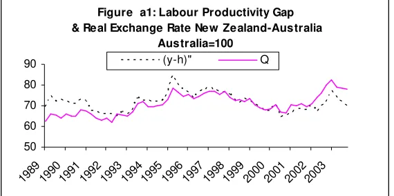
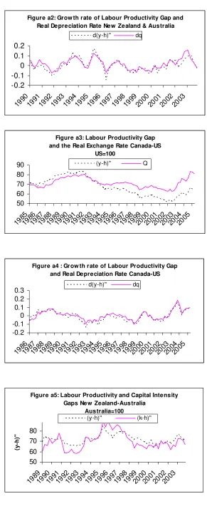
Data Appendix 1
Figures a1- a4 plot the labour productivity gap for New Zealand – Australia
and Canada – United States in log levels (y−h)t′′and in growth
ratesd(y−h)t′′.
2 The gap is defined as the log of the ratio of GDP per
hour-worked in the two countries, and the level of the real exchange rate defined in the text. We tried different measures of the real exchange rate and found no significant differences so we used the deviations from PPP. As defined in the
text, Yis real GDP, H is hour-worked, and Qis the deviation from PPP.
Lowercase denotes log and double prime on the variable denotes the gap between two countries’ magnitudes. The Australian data and the United States data are PPP-adjusted to the New Zealand and Canadian data such that Australia and the United States are set to 100. The levels have trends. The correlation is obviously very high.
In what follows a variety of tests for unit root such as the Dickey-Fuller, the
Augmented Dickey-Fuller, the Phillips-Perron test, Elliott(1999)and Perron
(1997) using a variety of specifications (different information criteria for testing lags, drift, drift and trend models) will be used. For GDP per hour worked and the real exchange rate, all tests failed to reject the unit root hypothesis in the level time series. Elliot’s test rejects the null more often than other tests, and especially in the case of the differenced data. Causality is much harder to test. Although the correlations are high one cannot tell at least by eyeballing the data which variables causes which. The HBS effect suggests that it runs from productivity to the relative price of nontradables or the real exchange rate, while Harris (2001) argues that the depreciation rate causes productivity gaps. We argued earlier that maybe causality runs both ways, and that both the productivity gap and the real exchange rate are affected by the same TFP shocks.
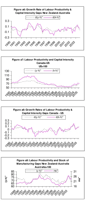
Figures a5-a8 plots the level and growth rates of labour productivity gap shown above against the level and growth rates of capital per hour-worked
gap(k−h)t′′andd(k−h)t′′. The stock of capital data are not readily available,
and especially at quarterly frequency. We use fixed capital formation expenditures instead as a proxy. The levels of capital intensity gaps in all countries have trends and the hypothesis of unit root could not be rejected by any of the tests statistics we reported earlier. The results do not vary with the specifications of these tests.
Figures a9-a12 plot the gap in the stocks of manufacturingµt′′and labour
productivity gap in levels, which we labelledmst′′and d(ms)t′′ and growth rates.
Visually, the correlations are striking in the case of New Zealand and Australia, but less so in the Canada – United States case. We tested the levels of the stock of manufacturing gaps in both New Zealand – Australia and
2
Canada – United States pairs for unit roots, and the hypothesis could not be rejected in all tests with many different specifications.
Figures a13-a16 plot the stock of R&D gaps ψt′′in levels, which we labelled
t
d
r ′′and growth rates d(rd′′)tagainst GDP per hour-worked gaps. We observe
downward trends in the R&D gap, New Zealand stock of R&D is much smaller than that of Australia and keeps falling, or Australia’s stock keeps increasing. For the Canada – United States case, the correlation is also visually clear. Canadian’s R&D stock must have picked up in 2003 as the trend is positive and sharp. The data have unit roots. The hypothesis could not be rejected by any of the tests outlined earlier.
The aging gapαt′′is plotted in figures a17-a20. Aging is the percentage of
workers age 55 and over in the labour force and the hypothesis was that this affects labour productivity adversely. Figures show negative (no clear
positive) correlation between ageing and labour productivity. The ratio is greater than1 for New Zealand; and is lower than 1 for Canada.
Figures a21-a24 plot the openness variable – total trade (imports plus
exports) as a percent of GDP gaps οt′′in levels and differences. New
Zealand’s trade exceed that of Australia. The correlation is pretty clear in the levels. The openness gap in the case of New Zealand – Australia is
stationary. All tests reject the null hypothesis that there is a unit root in the data.
Canada also trade more than US, as a percent of GDP, openness gap is correlated with labour productivity gap, trend downwards, but has a unit root.
[image:32.595.93.378.563.705.2]Figures a25-a28 plot the services’ productivity gap in levels and differences against the real exchange rate and the real depreciation rate. The data are annual indices taken from OECD website and interpolated to get quarterly data. The method is explained in the data appendix. The correlations appear negative as the theory would suggest and the data have unit roots. The Canada – United States data seem smoother.
Figure a1: Labour Productivity Gap & Real Exchange Rate New Zealand-Australia
Australia=100
50 60 70 80 90
198919901991199219931994199519961997199819992000200120022003