Clustered Graph Hierarchical Layout Algorithm
for Systems Biology Models
Pratik Erande
Research Scholar Vishwakarma Institute of
Technology, Pune
Noshir Tarapore
Assistant Professor Vishwakarma Institute of
Technology, Pune
Vrushali Inamdar
Software Team Lead Persistent Labs, Pune
ABSTRACT
In this article we describe a complete method to the layout clustered graph in hierarchical fashion. We have adopted Sugiyama[11] framework for hierarchical layout and modified its phases to produce the clustered graph layout. The algorithm is based on Sanders compound graph layout algorithm. Our main contribution is positioning of nodes with different sizes without any node overlap while maintaining straight lines for long edges. Experimental results show that the executiontime and quality of the produced drawings with respect to commonly accepted layoutcriteria are quite satisfactory.This algorithm is intended to integrate as a part of system biology software Cell-in-Silico, for drawing biological pathways with compartmental constraints and arbitrary nesting of graphs and molecular complexes.
General Terms
Data Visualization, Layout Algorithm.
Keywords
Clustered Graph, Hierarchical Layout, Biological Graphs, Node Size, Complex Species.
1.
INTRODUCTION
Graph structures are very useful to represent large data. The different comprehensive depictions of a graph can convey meanings and information to the viewer. The clustered graph conveys more information by capsulation of the nodes and edges in a cluster. These graphs are useful in many domains e.g. networking, system biology and finance. Automatically arranging nodes, edges and their clusters in human comprehensible form is called graph layouting. There are no strict rules about graph aesthetics, but generally accepted criteria are minimum edge crossings, shorter edge length and symmetry. In this article, we are going to focus on hierarchical layout of clustered graph.
In biology domain biologist need to analyze biological networks or pathway models. These models need to be visualized. Cell-in-Silico(www.cellinsilico.com), a comprehensive Systems Biology suite, is aimed at addressing the need of Experimental Biologists and Bioinformaticians for studying biological systems. The method we present is intended to use in Cell-in-Silico to layout clustered graphs. The graphs in biology domain are clustered graph and include special node type called ‘complex’. These nodes can include other nodes which forms the complex. For hierarchical graph edge orientation should be in downward direction. The nodes must be strictly drawn inside their respective cluster, similarly the clusters be drawn as per their actual nesting. To layout clustered graph properly is the motivation behind this project.
We present complete process to layout clustered graph in this paper.
The Sugiyama[11] has presented the framework for hierarchical graph layout process. This is a general model which describes the phases as (i) cycle removal (ii) layering the graph (ii) crossing reduction (iv) node positioning. Although this model is for a non-clustered graph, it become perfect with few additional steps to maintain cluster information while crossing reduction and positioning of nodes. This approach is taken by Sander[12]. Sander presents a method for layout of compound directed graph. In compound graphs a node can be a graph, thus nesting of graphs is allowed. The edges are allowed between combination of compound graphs and nodes. Clustered graph is similar to the compound graph but the edges are not allowed between graph and nodes. Sander[12] uses global partitioning into layers. The nodes are arranged on these layers such that border rectangles can be drawn without entangling with each other. This approach does crossing reduction by considering not only the edges within the subgraph but also edges connecting with nodes outside the cluster.
In step (iv) positioning of nodes phase; the ordering of nodes at layers must be maintained while assigning positions and the cluster rectangles must be drawn without an overlap with other nodes. Aesthetic criteria for readable graph include straightness of long edges, minimum edge slopes [1]. The long edges are divided by dummy nodes at each layer they cross. These long edges must be drawn as straight as possible. Previous approaches either optimize constrained objective function of coordinate differences or iteratively improve layout using one or various heuristics, or do both ([11][6][7][2][8][3][5][4][9][10]).We chose the Brandes[1] approach which is simplest among them with the lowest time complexity O(N) where N is total number of edges, dummy nodes and original nodes. This approach does not consider node height and width. This creates overlaps of nodes and false alignments. We have improved it to assign positions for nodes with different sizes without compromising the layout quality.
2.
CONVENTIONS
A directed graph G = (V,E) consist of set of nodes V and set of edges E. E is finiteset of ordered pairs over V. We denote an edge E from node u to v as uv, a path from u to v as u
A clustered graph G = (G’, T’) includes a directed graph G’= (V S, EG) and a tree T’ = (V S, ET),see figure 1b. Set V
contains leaf nodes of T’ which are called as graph nodes and set S contains the non-leaf nodes of T’ which are ‘subgraph’. G’ represents the edge connectivity between nodes and T’ represents a nesting relation of ownership between graph nodes and subgraphs. Thus T’ states that a subgraph may contain a subgraph or graph node. We say u belongs to w ∈ S iff w*u in T’. Layered graph G = (V D, E; L) is a graph G with a proper layering where set D contains the dummy nodes introduced for each subgraph. The edges are also called edge segments where edge source node is at layer Li and
target node is at layer Li+1. A layer contains nodes which are
at the same level from root node. The ordering of nodes at layer is described by left of relation ≺. If node u is left neighbor of v then it is denoted by u ≺ v and left(v) = u. For a given layered graph while assigning horizontal coordinates three margins are defined, γ is edge margin, β is node margin and δ is minimum separation between neighbor nodes at the same layer.
[image:2.595.321.538.238.402.2](a) Nesting Tree (b)Clustered Graph
Fig 1: Nesting Tree and Corresponding graph
3.
LAYERING
3.1
Preprocessing
The graph must be a DAG to apply the nest stages of algorithm. We remove cycles contained in graph. To find minimum number of edges to be removed is NP Complete problem. Instead we can use depth first search traversal of graph; the edges which discovers a node which is already visited, mark that edge as back edge. Reverse all back edges. This guarantees a cycle free graph, after layout restore all edges removed or reversed.
3.2
Global Layering
After preprocessing we have a clustered DAG G. The Layering process is dividing the graph nodes in layers. Uppermost layer is numbered 1. The process is to calculate rank of nodes; this rank value will decide which layer they belong to. In global layering we consider whole graph as a single hierarchy. The root node will reside at first layer in layered graph. The direct neighbor nodes of root node will be at second layer and so on. To make clustered DAG G as single connected hierarchy we create its copy - nested graph. Once a nested graph is created, all nodes of graph can be aassigned rank. The processes are as follows:
3.2.1
Nesting Graph
Nested graph [12] is a copy of original graph with all nodes reachable from a root node. The nodes we add for each
subgraph above and below all its nodes are called as border nodes.
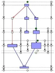
1. Assign upper and lower border nodes for each subgraph, see figure 2(b)
2. Add edges from upper border node to the nodes in subgraph. Add edges from all nodes in subgraph to the lower border node. These edges are called ‘nesting edges’.
3. Add ‘nesting edge’ from upper border node of subgraph to upper border nodes of its child subgraphs. Similarly from lower border nodes of child subgraphs to lower border node of subgraph 4. Add original graph edges and if an edge creates a
cycle then reverse it or delete it. The graph edges are denoted by dashed line, see figure 2(a).
[image:2.595.60.275.292.443.2](a) Nesting Graph (b)Graph
Fig 2: Nesting Graph and Corresponding graph with upper and lower border nodes
3.2.2
Ranking
Rank of node decides its vertical position relative to other vertices. The nodes with same rank forms a layer. One simple method to create proper ranks is to traverse graph topologically from root vertex. Upper border node of the nested graph is root node.
∈
The rank of a node decides its layer. Between two layers of graph nodes there can be a maximum 2k layers of border nodes, where k is the nesting depth of the graph[12]. Therefor assign rank value to the graph nodes in the multiple of 2k + 1. Assign upper and lower border nodes rank between multiples of 2k + 1. After the rank assignment from root upper border node, the lower border nodes are ranked close to the subgraph nodes it is connected to. Adjust upper border vertices to rank value closer to the subgraph node, it need one bottom up pass starting from lower border node to root node.
Let u be upper border node.
∈
3.2.3
Layering
Fig 3: Layers
3.3
Splitting Long Edges
The edges which cross one or more layers in layered graph are call long edges. We split the long edges at the points where they cross the layers by adding dummy node. So crossing reduction algorithm can guide these dummy nodes to produce reduced crossings by converting them to bends. This way when all the long edges are split by dummy node, every edge in thegraph will have source and target nodes at adjacent layers. This creates a proper hierarchy. Add dummy node to the nearest common parent graph in nesting tree T’. The graph in fig 3 has one long edge crossing graph nodes layer 14 and 21. Note that here we are not considering layer 20 and 27 to keep the number of dummy nodes less but we can split the edge at these layers too. Fig 4 shows graph after splitting a long edge.
Fig 4: Splitting long edge
4.
CROSSING REDUCTION
Crossing reduction will be done in two phases. Global crossing reduction: without considering the subgraphs nesting and Subgraph Crossing Reduction: considering the cluster bounding rectangles, to maintain node vicinity of nodes in same subgraph.
4.1
Global Crossing Reduction
We use barycenter crossing reduction heuristics. This is a two layer crossing reduction process. It is applied from top to bottom layer then bottom to top, this completes one iteration.
∈
Assign artificial positions to first layer and calculate barycenter weights of nodes at second layer. Reorder the
nodes at second layer in ascending order of their barycenter weights. The above equation is for top-down sweeps of the layered graph. Similarly use Successors of v in bottom-up sweeps in the above equation. This process might not remove all edge crossings but gives a good starting point for further Subgraph Crossing Reduction process.
4.2
Subgraph Crossing Reduction
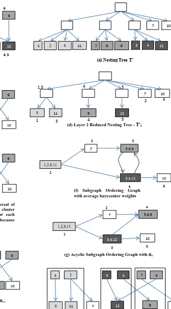
Global crossing reduction reduces some crossings but can reorder the nodes at layers which make subgraphs intertwined with each other [12]. To place nodes of same subgraph in an unbroken sequence at each layer we use reduced nesting trees. Reduced nesting tree for ith layer is nesting tree containing only nodes at layer i. This creates grouping of nodes of having same parent subgraph, see Figure 5(d).Each node v in reduced nesting tree is assigned average position of its direct and indirect child graph nodes. Sorted traversal on reduced nesting tree according to average position places the nodes at layer i with nodes of same parent subgraph in unbroken sequence. Though the nodes with the same subgraph placed in unbroken sequence, this sequence of subgraphs at each layer is not guaranteed to be the same for each layer in layered graph, so still two subgraphs can get intertwine. ‘z’ is integer for tweaking number iterations of crossing reduction process.
Algorithm 1: Crossing Reduction Input: Nesting Tree T’, Layered Graph L A 0 //Average crossings in z iterations C current crossings
while A ≠ C do
Assign artificial positions to layer 1 foreach Li∈ L , i = 1 to |L| do
foreach v ∈ Li do
calculate barycenter for v end
Sort Li nodes by their barycenter weight
Sorted traversal of Ti’ according reordered Li
end
Create subgraph ordering graph OG foreach v ∈ T’ do
update average barycenter for v end
Break cycles and sort OG topologically Calculate αo,1
Sorted traversal of Ti’ according to αo,1
foreach Li∈ L , i = 1 to |L|
foreach v ∈ T’ do
update average barycenter for v end
Calculate αo,i
Sorted traversal of Ti’ according to αo,i
end
..Similarly do bottom-up traversal.. Update A and C
[image:3.595.118.215.423.565.2]Fig 5: Crossing reduction top-down iteration (b) Layered Graph with barycenter
weights at layer 2
(a) Nesting Tree T’
1 2 3 4 5 6
8 7 11 9 12 10
(c) Layer 2 sorted according to barycenter weights
1 2 3 4 5 6
8 11 7 9 12 10
(e) Layer 2 according to sorted traversal of reduced nesting tree. Nodes of same cluster are placed in unbroken sequence at each layer. Subgraph are still intertwined because of 9 and 12
(d) Layer 2 Reduced Nesting Tree - T’2
7
8 9
10
11 12
6
1.5 4 5
5 4
1 3
2
(f) Subgraph Ordering Graph with average barycenter weights
(g) Acyclic Subgraph Ordering Graph with o
1 2 3 4 5 6
8 11 7 12 9 10
1 2 3 4 5 6
8 11 7 12 9 10
(h) Layers sorted according to o,i
(i) Placement of nodes after one top to down iteration in Clustered Graph
1,2,8,11
7 5,6,9
3,4,12 10
1
2 4
3 5
1
7
2 8 5 6 9 3 4
10
11 12
1 2 3 4 5 6
8 12
7 9 10 11
2 1 4 5 2 4.5 1 2 3 4 5 6
1,2,8,11
7 5,6,9
3,4,12 10
2
3 5
To place all subgraphs in same sequence at each layer SubgraphOrdering Graph is used [12]. Subgraph ordering graph represents subgraph/node is left to which subgraph/node. If a node v is direct left neighbor of node u on the same layer we add edge in nearest common parent of node v and u. See Figure 5. If any subgraphs are intertwined then there will be a cycle in subgraph ordering graph. Remove cycles by breaking them at node with minimum average barycenter weight, as shown in Figure 5. A topological traversal of subgraph ordering graph gives ordering αo,
denoting which subgraph is to the left of other subgraph.
5.
POSITIONING
[image:5.595.123.211.284.402.2]The edge crossings are reduced and nodes are placed according to their subgraphs at each layer. Now we need to calculate absolute positions for graph nodes such that there will be enough space to draw subgraph boundaries. To draw subgraph vertical boundaries straight we aadd trail of dummy vertical nodes one to the left and one to the right side of each layer in every subgraph.
Fig 6: Vertical Dummy Nodes for every subgraph
The goal is to position the long edges as straight as possible and vertical borders of subgraph strictly vertical without reordering the nodes at any layer. We present a heuristic approach based on Brandes [1] approach. The nodes have different height and width. There should be no overlap between any two nodes and node and subgraph boundary. The process consists of three steps. The first and second steps are carried out four times. The first algorithm referred as vertical alignment, to align nodes with eitherits median upper or median lower neighbor node. This will give maximum possible straight long edges positions in upward and downward direction. The alignment conflicts are resolved with leftmost and rightmost direction. Combination of the directions creates four alignments namely Upward-Left, Upward-Right, Downward-Left and Downward-Right. In second step each alignment is given absolute positions according to four alignments. In the last step these alignments are balanced and merged to produce final absolute positions of nodes and subgraph borders. We have givenalgorithmfor upward left alignment deriving the other three alignments is symmetric.
5.1.1
Mark Edge Conflicts
Hierarchy of nodes might contain edge crossings. Every edge crossing is referred to as edge conflict. The inter-cluster edge crosses with at least one vertical border edge. To give preference to edge to be drawn vertically straight over its conflicted edges we mark other edges as conflicted. If conflict is between graph edge and long edge, mark the graph edge as conflicted [1]. In addition to that if graph edge is conflicted with vertical border edge then graph edge is marked similarly long edge is marked when conflicted with vertical border edge.
5.1.2
Vertical Alignment
We want to align nodes with their median upper side neighbor for positioning the long edges as straight as possible and resolve alignment conflict by placing nodes in left alignment. The alignment is stored in cyclic linked list implemented in an array of size of total number of graph nodes. The set of vertically aligned nodes are called ‘blocks’ [1]. Every node in block points to its block’s first node i.e. root node. A block root node can be aligned to next node below it; similarly next node aligned to its next node, this link goes on till the last node of the block which is then aligned to the root node. The node in block has to be assigned a same x coordinate i.e. same absolute horizontal position to draw a straight edge.
Algorithm 2: Upward Left Alignment Input: Layered Graph L
initialize root[v] v, v ∈ V S initialize align[v] v, v ∈ V S for i 1,...,|L| do
p -∞;
for v 1,...,|Li| do
if v has upper layer neighbors u1≺u2≺..≺ud with d > 0
then
for m do if(align[v] = v)then
if(edge(um , v) is not marked as conflicted)then
if(p<pos[um])then
align[um] v;
root[v] root[um];
align[v] root[v]; ppos[um];
end end end end end end end
//Align vertical border nodes visited[v] F, v ∈V S foreach v ∈ V S do
if(visvertical border node)then if(visited[v] = F)then while(predecessor(v) ≠∅)do visited[v] T;
v predecessor(v); end
rv;
while(successor(v) ≠∅)do align[v] successor(v); root[v] r;
v successor(v); end
align[v] r; root[v] r; end
5.1.3
Horizontal Compaction with Node sizes
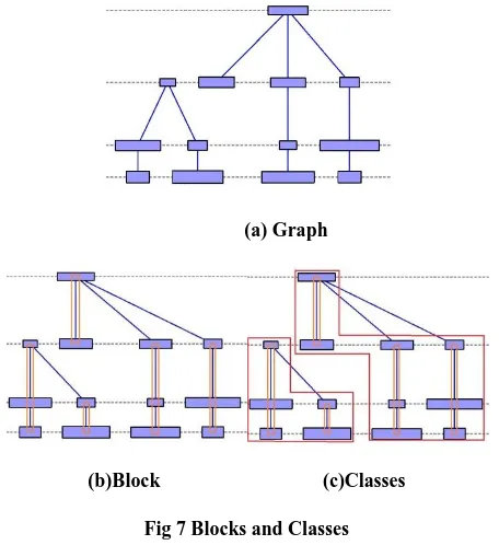
In the second step of positioning, the horizontal coordinates are assigned to the nodes according to the four node alignments. All the nodes in the same block are assigned coordinate of their block root node. This way it guarantees the nodes aligned to each other will be drawn vertically in a straight line. If we consider an edge from every node to its next aligned node in a block and its predecessor on the layer except edge from the bottom node to block’s root node, see figure 7. This will create a DAG, the root of blocks will be sink and always there will be at most only one node of this kind at each layer. We partition this graph into ‘classes’. The class of block is the reachable sink which has topmost root [13]. The algorithm places the classes with minimum separation calculated from the node widths and the maximum position of predecessor class node. We have corrected the original algorithm of horizontal compaction from Brandes [1] paper and added horizontal size considerations in the process. The constants for edge margin and node margin can be varied.
(a) Graph
[image:6.595.54.282.279.528.2](b)Block (c)Classes
Fig 7 Blocks and Classes
Algorithm 3: Horizontal Compaction with Node Sizes function space(v)
begin s 0;
if (v is DummyNode) then s width[v] + γ; else
s width[v] + β; end
ss / 2; returns; end
functionplace_block(v) begin
if (x[v] = undefined) then x[v] 0;
u v; repeat
if(pos[u] > 1)then r root[left[u]]; place_block(r);
if(sink[v] = v)then sink[v] sink[r]; end
δ space(left[u]) + space(u); if(sink[v] ≠ sink[r])then
ShiftClass[sink[r]] [sink[v]]
min{ShiftClass[sink[r]][sink[v]] , x[v] - x[r] –δ}; else
x[v] max{x[v] , (x[r] + δ)}; end
end
u align[u]; until(u = v); end
end
initialize ShiftClass[v][u] ∞, v ∈ V S , u ∈ V S initialize sink[v] v , v ∈ V S;
initialize shift[v] ∞, v ∈ V S; initialize x[v] undefined, v ∈ V S; //Root coordinate relative to sink forech v ∈ V S do
if root[v] = v then place_block(v); end end
foreach layer Li∈ L do
foreach v ∈ Lido
if(left(v) ≠ ∅)then x[v] x[root[v]];
if(v = root[v] and v = sink[v])then minShift ∞;
foreach u ∈ShiftClass[v]do if(shift[u] < ∞)then
minShift min{ shift[u] + ShiftClass[v][u], minShift};
end end
shift[v] minShift; end
end end end
foreach layer Li∈ L do
foreach v ∈ Lido
if(shift[sink[ root[v]]] < ∞)then x[v] x[v] + shift[sink[root[v]]]; end
end end
5.1.4
Merging Alignments
[image:6.595.51.280.284.758.2](a) Upward Left (b) Upward Right
(c) Downward Left (d) Downward Right
[image:7.595.85.251.67.502.2](e) Balanced Alignment
Fig 8: Four alignments and final balanced alignment
5.1.5
Y Coordinate Assignment
In y coordinate assignment there are two node properties which we taken into account: node height and its edge degrees. It is obvious if the node heights are not uniform then layers must be placed such that the nodes must not overlap vertically. If nodes have more out (in) degree then next (previous) layer must be placed at more distance apart from each other to minimize the edge slope.
6.
RESULTS& ANALYSIS
[image:7.595.311.532.78.224.2]In this section we present the performance statistics. Figure 9 shows the performance in terms of time for graphs with different number of nodes. Each graph sample contains same number of cluster and constant nodes to edge ratio. The graph obtained is fairly linear. This proves the algorithm has a linear time complexity till 1100 nodes graph.
[image:7.595.312.546.262.348.2]Fig 9: Performance of algorithm Nodes vs. Time
Table 1: Impact of long edges
Nodes Edges Cluster Long
Edges
Time (ms)
60 55 7 12 219
60 55 7 22 296
60 55 7 31 337
60 55 7 40 393
The table 1 shows the performance in terms of time to complete the layout. The graph used has same number of nodes, clusters and edges. We only vary the number of long edges. The long edges are forward edges in the graph. The time required to layout increases as the number of long edges increase. This is because the long edges are split at layers they cross. It increases the number of dummy nodes hence increases the time to layout.
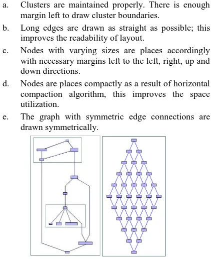
The figure 9 shows output of our graph layout algorithm. These two graphsexpose the features of our method:
a. Clusters are maintained properly. There is enough margin left to draw cluster boundaries.
b. Long edges are drawn as straight as possible; this improves the readability of layout.
c. Nodes with varying sizes are places accordingly with necessary margins left to the left, right, up and down directions.
d. Nodes are places compactly as a result of horizontal compaction algorithm, this improves the space utilization.
e. The graph with symmetric edge connections are drawn symmetrically.
(a)Clustered Graph (b) Symmetric Graph
Fig 9: Output Graphs
0 1000 2000 3000 4000 5000 6000
Ti
m
e
in
m
il
li
se
co
n
d
s
[image:7.595.331.542.463.721.2]Figure 10(b) was produced by our layout method and figure 10(a) shows the hierarchical layout of same graph from systems biology software Cell-Designer 4.2 [14]. The difference in layering creates unnecessary edge routing in graph figure 10(a) and violation of feature a, on the other side our layout draws cluster lines inside the proper cluster. Thus creates more comprehensible layout.
(a) Cell Designer Graph Layout (b) Our method layout
Fig 10: Output Graphs
7.
CONCLUSION
The presented algorithm gives good results, is flexible and fully automatically layouts the clustered graphs i.e. it does not need user intervention. It is well suited for the layout of clustered graphs such as biological networks.
The global layering improves the space utilization. The horizontal compaction method is an added advantage implemented in this method, nodes with different sizes are placed compactly to improve the horizontal space utilization. The barycenter method used in combination to the subgraph ordering graph method gives good crossing reduction. This method is applied on globally partitioned graph, we can extend this by using crossing reduction method which considers the subgraph even at globally partitioned layers. There are several generic elements present in given methodlike different layering techniques, in positioning break conflicts in favor of high degree vertices etc., which can be further used to get any domain specific features in graph layout.
8.
ACKNOWLEDGMENTS
This research project is funded by Persistent Labs, Pune, we are thankful to them. We thank Vivek Kulkarni for his critical comments and suggestions during the project. We are grateful to our jury Dr. S. T. Patil for his comments and suggestions. Our friends and colleagues Anwar Shaikh, Pratham Shah and Ujwala Bangar at Labs have provided good suggestions on implementation, we are thankful to them. We are thankful to Mayur Narkhede for all the discussions and criticisms on algorithms he generously offered whenever asked for.
9.
REFERENCES
[1] Ulrik Brandes and Boris Kopf, 2002. “Fast and Simple Horizontal Coordinate Assignment”. 9th international symposium on Graph Drawing(GD’01) (LNCS 2265), 31-44.
[2] Peter Eades, Xuemin Lin, and Roberto Tamassia, 1996.“An Algorithm for Drawing a Hierarchical Graph”. International Journal of Computational Geometry & Applications, 6:145-156.
[3] Peter Eades and Kozo Sugiyama, 1990. “How to Draw a Directed Graph”. Journal of Information Processing, 13(4), 424-437.
[4] Michael Frohlich and Mattias Werner, 1994.“The graph visualization system daVinci - a user interface for applications”. Technical Report 5/94, Department of Computer Science, University of Bremen.
[5] Emden R. Gansner, Eleftherios Koutsofios, Stephen C. North, and Kiem-Phong Vo.,1993.“A Technique for Drawing Directed Graphs”. IEEE Transactions on Software Engineering, 19(3):214-230.
[6] Emden R. Gansner, Stephen C. North, and Kiem-Phong Vo., 1988. “DAG - A Program that Draws Directed Graphs”. Software - Practice and Experience, 17(1):1047-1062.
[7] Georg Sander, 1995. “Graph Layout through the VCG Tool”. In Roberto Tamassia and Ioannis G. Tollis, editor, Proceedings of the DIMACSInternational Workshop on Graph Drawing (GD ’94), LNCS 894, 194-205, Springer. [8] Georg Sander, 1996. “A fast heuristic for hierarchical
Manhattan layout”. In Franz J. Brandenburg, editor, Proceedings of the 3rd International Symposium on Graph Drawing (GD ’95), LNCS 1027, 447-458. Springer.
[9] Georg Sander, 1999. “Graph Layout for Applications in Compiler Construction”. Theoretical Computer Science, 217(2):175-214.
[10] Kozo Sugiyama and Kazuo Misue, 1991. “Visualization of Structural Information: Automatic Drawing of Compound Digraphs”. IEEE Transactions on Systems, Man and Cybernetics, 21(4):876–892.
[11] Kozo Sugiyama, Shojiro Tagawa, and Mitsuhiko Toda, 1981. “Methods for Visual Understanding of Hierarchical System Structures”. IEEE Transactions on Systems, Man and Cybernetics, 11(2):109–125.
[12] Georg Sander, 1996. “Layout of Compound Directed Graphs”. Technical Report A/03/96. Sarland University, D-66123 Saarbrücken, Germany.
[13] Christoph Buchheim, Michael Jünger, and Sebastian Leipert, 2001. “A Fast Layout Algorithm for K-Level Graphs”. In Joe Marks, editor, Proceedings of the 8th International Symposium on Graph Drawing (GD 2000), LNCS 1984, 229–240, Springer.
[image:8.595.59.278.152.241.2]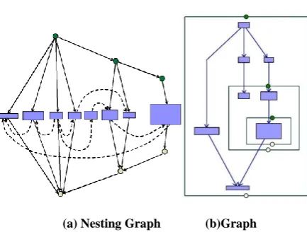

![Figure 10(b) was produced by our layout method and figure 10(a) shows the hierarchical layout of same graph from systems biology software Cell-Designer 4.2 [14]](https://thumb-us.123doks.com/thumbv2/123dok_us/8042249.771715/8.595.59.278.152.241/figure-produced-layout-hierarchical-systems-biology-software-designer.webp)
