Designing Spam Model Classification Analysis using Decision Trees

(1)

Designing Spam Model- Classification Analysis using

Decision Trees

Shweta Rajput

Assistant Professor, CSE,Chitkara University, India.

Amit Arora

Assistant Professor, CSE,Chitkara University, India.

ABSTRACT

A spam has diluted the message pool, causing frustration so require an automatic processing of emails. This study is to construct a spam model using classification technique in data mining. To accomplish this, experiments were conducted on spam dataset downloaded from the UCI machine learning repository which was classified using a popular data mining tool called WEKA. The final classification result should be „1‟ if it is finally spam, otherwise, it should be „0‟.Email is popular mode of communication and its users are growing day by day. But, due to social networks and electronic business, most of the emails contain unsolicited bulk e-mail called spam. Several solutions have been proposed to overcome the spam problem, filtering using decision tree classifiers is the one of the most significant techniques. Machine learning classifiers, J48, J48graft and Simple CART were used for classifying spam messages from e-mail. These trees are induced first and then prune sub trees to improve classification accuracy and size of tree. It helps to reduce size, complexity and to achieve better predictive accuracy of final classifier. Grafting is then applied as a post process to an inferred decision tree. Results showed that J48graft had pretty good prediction accuracy as compared to CART and J48 algorithms.

Keywords

Weka, Simple CART, J48, J48graft, Spam filtration, Post pruning, Pre pruning, Classification, Grafting

1. INTRODUCTION

The "spam" concept is diverse, it is used for advertising products/web sites, make money fast schemes and pornography and act as a prime medium for phishing of sensitive information and to spread malicious software to various users. With the extensive use of internet, e-mail is proved as best mode of information exchange. However spam email has degraded the proficient usage of emails. Mailboxes of millions of users get cluttered with junk mails which then results in delay in delivery of legitimate mail and may result in deleting important mail by mistake. Spam Classification in data mining find out a model for class attribute as a function of values of other attributes. It classifies an incoming message into predefined categories based on contents of a message. The spam filtering using decision trees will move out unsolicited e-mails automatically from a user's mail stream. In this paper decision tree is used as classifier. Decision tree induction is top down process. Root is selected using attribute selection measures like information gain, gini index and gain ratio and so on. To derive a prediction, a test instance is

filtered down the tree, starts from the root node, until it reaches a leaf. For every node one of instance‟s attribute is tested, and the instance is propagated to branch that corresponds to the final result of the test. The prediction is the class label that is attached to leaf. But, it suffers from the problem of overfitting to the training data, resulting in low predictive power for previously unseen data. Pruning can be used as a tool to correct for potential overfitting.It is a technique that reduces size of decision tree by removing sections of decision tree that provide little power to classify instances[1]. This paper covers two types of pruning, pre pruning and post pruning and grafting. This paper presents extension to decision tree grafting that dramatically reduce induction time, reduce the complexity of inferred trees and raise prediction accuracy. There are a variety of algorithms for building decision trees and frequently used over the years are C4.5 [5] and ID3.

Sections II outline classifications approach and attribute selection measures. In section III post pruning and pre pruning techniques are discussed with their methods. Section IV dataset description and machine learning tool WEKA with various pruning factors in weka interface like confidence factor, Minimum no of objects, No of folds (reduced error pruning).Section V outlines result and discussion. Section VI represents conclusion.

2. METHODOLOGY

In this paper, J48, Simple CART and J48graft decision tree learning algorithms were used for analyzing the dataset and to predict the performance. The decision tree consists of three elements, root node, internal node and a leaf node. At top level is the root node. Leaf node is the terminal node and the nodes in between is called the internal node. Each internal node denotes test on an attribute, each branch refers to an outcome of the test, and each leaf node tells about a class label. The decision tree is constructed based on "Divide and Conquer". The nodes are chosen from the top level based on quality attributes such as Information Gain, Gain Ratio, Gini Index etc. The main motivation for different classification algorithms is accuracy improvement for the spambase dataset. Different classification methods used are CART, J48graft and J48 decision tree algorithm.

2.1 J48 CLASSIFIER

(2)

named as C4.5 algorithm in the WEKA. It generates non binary tree and uses measure called gain ratio to construct decision tree, the attribute with highest normalized gain ratio is taken as the root node and the dataset is split based on the root element values[8]. Again the information gain is calculated for all the sub-nodes individually and the process is repeated until the prediction is completed. C4.5 is an evolution and refinement of ID3 that accounts for missing data values, continuous attribute value ranges, and pruning of decision trees and so on. Error–based pruning is performed after the growing phase. J48 can handle both continuous and discrete attributes, training data with missing attribute values and attributes with differing costs and provide an option to prune trees after creation. There are a number of parameters related to tree pruning in the J48 algorithm and should be used with care as they can make a noteworthy difference in the quality of results. J48 employs two post pruning methods, namely subtree replacement and subtree raising.

2.2 J48GRAFT CLASSIFIER

J48graft generates a grafted DT from a J48 tree. The grafting technique adds nodes to an existing decision tree with the purpose of reducing prediction errors. These algorithm identifies regions of the instance space that are not occupied by training instances, or occupied only by misclassified training instances, and consider alternative classifications for those regions. In other words, a new test will be performed in the leaf, generating new branches that will lead to new classifications. Grafting is an algorithm for adding nodes to the tree as a post-process. Its purpose is to increase the probability of rightly classifying instances that fall outside the areas covered by the training data. Grafting is a post-process that can be applied to decision trees. Its aim is to decrease prediction error by reclassifying regions of the instance space where no training data exists or where there is only misclassified data. Its aim is to find the best matched cuts of existing leaf regions and branches out to create new leaves with other classifications than the original. Though tree becomes more complex, but here only branching that does not introduce any classification errors in data already rightly classified is considered. Newly generated tree thus reduce errors instead of introduce them.

2.3 CART CLASSIFIER

Classification And Regression Trees algorithm is a data prediction algorithm based on binary Recursive partitioning. CART uses learning sample which is a set of historical data with pre-assigned classes for all observations for building decision trees. The splits are selected using the gini-index criteria and the obtained tree is pruned by cost–complexity Pruning. CART bifurcate data into two subsets so that the records within each subset are more homogeneous than in the previous one. It is a recursive process – each of those two subsets is then split again, and the process is repeated until the homogeneity criterion is reached or until another stopping criterion is satisfied. The same predictor field may be used several times at different levels in the tree. It uses surrogate splitting to make the best use of data with missing values. It takes account of both the number of errors and the complexity of the tree. The size of the tree is used to represent the complexity of the tree[9].

2.4 Attribute Selection Measure

During model building process, inclusion of inappropriate, superfluous and noisy attributes can result in poor predictive performance and increased computation. The aim of attribute

selection is to search for a best set of attributes to improve classification accuracy in model construction.

2.4.1 Gain Ratio Attribute ranking

C4.5 uses gain ratio as attribute ranking measure[8]. The attribute with the maximum gain ratio is selected as the splitting attribute. The split information value represents the potential information generated by splitting the training data set D into v partitions corresponding to v outcomes on attribute A

SplitInfoA (D)=- DJ D ∗ log2(

|Dj | |D|) V

j=1

Gain Ratio is calculated as:

Gain Ratio (A) = Gain (A) / SplitInfo(A)

2.4.2 Gini Index Attribute ranking

The Gini Index (used in CART) measures the impurity of D, data partition as

Gini(D)=1- mi=1pi2

Where m is the number of classes and pi is the probability that a tuple in D belongs to class Ci.

3. PRUNING METHODS FOR

DECISION TREES

Even though the decision tree generated by the J48, J48graft was accurate and efficient, but they result in bulky trees leading to problem of overfitting [10]. Overfitting results in decision trees that are more complex than necessary. Pruning is required to obtain small and accurate models, avoids unnecessary complexity and helps in optimizing the classification accuracy. Pruning prevent overfitting to noise in data. There are two strategies for pruning, pre-pruning and post-pruning. Post-pruning is preferred in practice as pre pruning can stop early. Another key motivation of pruning is ”trading accuracy for simplicity” as presented by Bratko and Bohanec[4]. When the goal is to produce a sufficiently accurate compact concept description, pruning is highly useful.

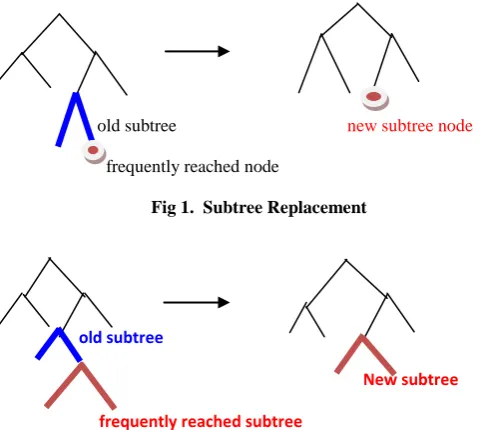
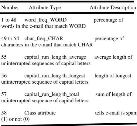
3.1 Post-pruning

(3)

node, tree is considered for replacement once all its subtrees have been considered.

old subtree new subtree node

[image:3.595.37.279.106.321.2]

frequently reached node

Fig 1. Subtree Replacement

old subtree

New subtree

frequently reached subtree

Fig 2. Subtree Raising

3.1.1 Reduced error pruning

It is a post-pruning method used by J48 algorithm that divides dataset into three parts, namely training set, testing set and hold-out set (Pruning set). It uses a hold-out set (a fraction of the training data) for making pruning decisions and to estimate generalization error. So less data is used to determine the whole structure of the tree as compare to other pruning methods. However, once the structure has been summarized, the full training data can be back-fitted against the structure in order to find the node and leaf class distributions. Node is then replaced with its majority classification. If the performance of the modified tree is just as good or better on the validation set as the current tree then set the current tree equal to the modified tree.Subtree is then replaced by leaf node, means pruning is done. Nodes are removed only if the resulting tree performs no worse on the validation set. Nodes are pruned iteratively, at each iteration the node whose removal most increases accuracy on the validation set is pruned [6]. Pruning stops when no pruning increases accuracy. The problem with this approach is that it potentially “wastes” training data on the validation set, reducing the amount of data available for training. If test set is smaller than training set, it may lead to overpruning but it has the advantage of simplicity and speed. The popular C4.5 algorithm adds to the reduced error based pruning method the subtree replacement operator. Numfold parameter is used to achieve reduced error pruning.

3.1.2 Cost complexity pruning

Simple cart employs cost-complexity pruning. It is a two step algorithm. In the ﬁrst stage, a sequence of trees T0, T1,. . . ,Tk is built on the training data where T0 is the original tree before pruning and Tk is the root tree. In the second stage, one of these trees is chosen as the pruned tree, based on its generalization error estimation. On training examples, initial tree has no errors, but replacing subtrees with leaves increases errors. It finds cost-complexity, a measure of average error reduced per leaf. As pruning is based on misclassification rate so it calculates number of errors for each node if collapsed to leaf.

Error Rate of a node r(t) is calculated as:

err (t)=# 𝑜𝑓 𝑒𝑥𝑎𝑚𝑝𝑙𝑒𝑠 𝑚𝑖𝑠𝑠𝑐𝑙𝑎𝑠𝑠𝑖𝑓𝑖𝑒𝑑 𝑖𝑛 𝑛𝑜𝑑𝑒_{# 𝑜𝑓 𝑎𝑙𝑙 𝑒𝑥𝑎𝑚𝑝𝑙𝑒𝑠 𝑖𝑛 𝑛𝑜𝑑𝑒}

P(t) is Probability of Occurrences of a node

p(t)=# 𝑜𝑓 𝑒𝑥𝑎𝑚𝑝𝑙𝑒𝑠 𝑖𝑛 𝑛𝑜𝑑𝑒_{# 𝑡𝑜𝑡𝑎𝑙 𝑒𝑥𝑎𝑚𝑝𝑙𝑒𝑠}

Error Cost of a node is given as:

R(t)=err(t)*p(t)=# 𝑜𝑓 𝑒𝑥𝑎𝑚𝑝𝑙𝑒𝑠 𝑚𝑖𝑠𝑠𝑐𝑙𝑎𝑠𝑠𝑖𝑓𝑖𝑒𝑑 𝑖𝑛 𝑛𝑜𝑑𝑒_{# 𝑡𝑜𝑡𝑎𝑙 𝑒𝑥𝑎𝑚 𝑝𝑙𝑒𝑠}

If node t was unpruned then error cost of subtree, T rooted at t:

R(t)= 𝑖=𝑛𝑜 𝑜𝑓 𝑙𝑒𝑎𝑣𝑒𝑠𝑅(𝑖)

The error complexity of the node is calculated using following equation:

a(t)=_{𝑛𝑜 𝑜𝑓 𝑙𝑒𝑎𝑣𝑒𝑠 −1}𝑅 𝑡 −𝑅(𝑇)𝑡

where a measures the VALUE of corresponding subtree.

The method consists of following runs:

 a was computed for each node.

 the minimum a node is pruned.

 above is repeated and a forest of pruned tree was formed.

 Finally tree with optimum accuracy was selected.

3.2 Pre-pruning

Generating a smaller and simpler tree with fewer branches and while building keep on checking whether tree is overfitted or not is known as pre-pruning. It stop growing a branch when information becomes unreliable and is based on statistical significance test.Pre pruning techniques include minimum no of object pruning and chi square pruning.

3.2.1 Minimum no of object pruning

The minObj parameter means minimum no of object per branch is available in Weka in J48 and J48graft.This option tells c4.5 limit the minimum number of examples each leaf could have and not to create a new tree branch unless that branch contains greater than or equal to specified number of instances. This prevents overfitting of data when number of instances remaining to be classified is small. This parameter is varied in J48, J48graft algorithm to test predictive accuracy. If split result in child leaf that denotes less than minobj from dataset, parent node and children node are compressed to a single node.

(4)

4. DATASET DESCRIPTION AND

MACHINE LEARNING TOOL

4.1. Dataset Used

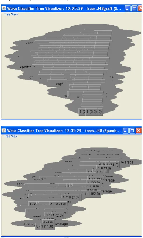
Experiments were conducted on spam dataset downloaded from the UCI machine learning repository, http://www1.ics.uci.edu/~mlearn/MLRepository.html[7] for analysing the decision tree classifiers using WEKA data mining tool. SpamBase data set was collected internally by Hewlett Packard Labs for research purposes and then released to the public. There are many features present in the body of the-mail message that may indicate spam. Recognizing this from the features present in the body of an e-mail is hard, as these features are not globally constant, they would vary not only from spammer to spammer, but from user to user. The numbers of attributes are 58 out of which 57 are continuous and 1 has nominal class label. Most of the attributes indicate whether a particular word or character was frequently occurring in the e-mail.

Definitions of the attributes are given as:

Number Attribute Type Attribute Description

1 to 48 word_freq_WORD percentage of words in the e-mail that match WORD

49 to 54 char_freq_CHAR percentage of characters in the e-mail that match CHAR

55 capital_run_leng th_average average length of uninterrupted sequences of capital letters

56 capital_run_leng th_longest length of longest uninterrupted sequence of capital letters

57 capital_run_leng th_total sum of length of uninterrupted sequence of capital letters

58 Class attribute tells e-mail is spam (1) or not (0)

48 continuous real attributes of type word_freq_WORD, i.e. 100 * (number of times the WORD appears in the e-mail) /total number of words in e-mail. A ‟word‟ in this case is any string of alphanumeric characters bounded by non alphanumeric characters or end-of string. Six continuous real attributes of type char_freq_CHAR denotes percentage of characters in the e-mail that match CHAR, i.e. 100 * (number of CHAR occurrences) / total characters in e-mail. The runlength attributes (55-57) measure the length of sequences of consecutive capital letters. The last column of 'spambase.arff' denotes whether the e-mail was considered spam (1) or not (0).Missing Attribute Values are none.

Class Distribution for 4601 instances:

SPAM 1813 39.40%

HAM 2788 60.60%

4.2. Data Mining Tool

To construct the spam model, WEKA (Waikato Environment for Knowledge Acquisition) tool version 3.6.9 which is available from http://www.cs.waikato.ac.nz/ml/weka was downloaded and is used for evaluation purpose. WEKA is open source machine learning software implemented in JAVA.Weka tool reads ARFF (Attribute Relation File Format), so, file which is downloaded from UCI repository is first converted into ARFF File Format. Under the decision tree method in WEKA, classification experiment is performed with 3 algorithms,which were J48,J48graft and Simple Cart.

 binarySplits: It split numeric attribute into 2 ranges using an inequality.

 confidenceFactor: smaller values(means we have less confidence in training data)will lead to more pruning as it filter out irrelevant nodes.

 minNumObj: tells minimum number of instances per leaf node

 numFolds: calculates the amount of data for reduced error pruning – one fold used for pruning, the rest for growing the tree.

 reducedErrorPruning: parameter tells whether to apply reduced error pruning or not.

 subtreeRaising: whether to use subtree raising during pruning.

 Unpruned: whether pruning takes place at all. Value is change to "True" to build a pruned tree in c4.5.

 useLaplace: whether to use Laplace smoothing at leaf node.

5. RESULT EVALUATION

[image:4.595.52.278.288.496.2]

(5)

5.1 Using 10-Fold Cross Validation

TABLE1

UNPRUNED TREE RESULT

Parameters J48 J48graft Simple Cart

Total instances 4601 4601 4601

Correctly classified

4260

4291 4268

Incorrectly classified

341

310 333

Kappa statistic 0.8448 0.8586 0.8481

Mean absolute error

0.0836 0.0776

0.0963

Root mean square error

0.2612 0.2521

0.2583

Time taken to build model

4.75 sec 5.06 sec

0.97 sec

Numbers of leaves

190 676

114

Accuracy 92.58% 93.26% 92.76%

Size of Tree 379 1351 227

TABLEII

PRUNED TREE RESULT

5.2 Using Percentage Split with Training

Data Being 66% and the Rest is Testing

Data

For each algorithm percentage split test was used, data set was bifurcated into a training part and a test part. For the training set 66% of the instances were used in the data set and remaining part was used as test set. Performance of the classifiers tested using 66% split test option are summarized in the table 3(Unpruned) and table4 (Pruned).

TABLE3

Unpruned Tree Result

Correctly classified 1440 1443 1438

Incorrectly classified 124 121 126

Kappa statistic 0.8347 0.8379 0.8308

Mean absolute error 0.0895 0.088 0.1083

0.2665 0.2672

0.2717

4.78 sec 5.11

sec

0.84

sec

Numbers of leaves 190 676 114

Accuracy 92.07% 92.26% 91.94%

TABLE4

Pruned Tree Result

Kappa statistic 0.8358 0.8501 0.8279

0.2686 0.2588

0.2722

4.83sec 5.14 sec 5.2 sec

Accuracy 92.19% 92.90% 91.81%

Kappa statistic 0.8528 0.8589 0.841

0.2562 0.2513

0.2606

6.19sec 6.55 sec 5.63 sec

Accuracy 92.97% 93.28% 92.43%

(6)

5.3. Measuring Performance: Precision and

Recall

A well employed metric for performance measurement in information retrieval is precision and recall. Recall is the proportion of relevant items that are retrieved, which in this case is the proportion of spam messages that are actually recognized. In the spam classification context, precision is the section of the spam messages classified as spam over the total number of messages classified as spam. Accordingly if only spam messages are classified as spam then the precision is 1.If a good legitimate message is classified as spam, the precision will drop below 1.It is more important for the precision to be at a high level than the recall rate. Incorrectly classified instances signify that some mails have either been categorized as FP (false positive) or as FN (false negative).FP means ham has been categorized as spam and FN means spam has been categorized as ham.

[image:6.595.311.556.70.427.2]

From Table I, II, III and IV it is seen that, J48graft algorithm excel other two algorithms. The grafting algorithm takes into account instances outside the analyzed leaf (global information) while pruning only looks at instances within the analyzed leaf (local information).

[image:6.595.315.555.72.252.2]

Fig 3. The top figure is the tree structure for J48 and the bottom figure is the tree structure for grafted J48.

[image:6.595.313.556.275.429.2]

Fig 4. Accuracy vs Decision tree unpruned classifiers

Fig 5. Accuracy vs Decision tree Pruned classifiers

Fig 4 and Fig 5 shows comparison of three unpruned and three pruned classifiers. It is clear from figures that J48graft outperforms in both cases in terms of accuracy.

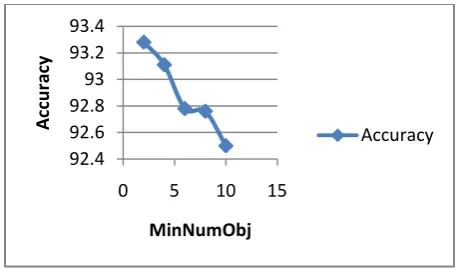
Fig 6. Minnumobj vs tree size in pruned J48graft classifier (Confidence factor was held constant 0.25 and 10

fold cross validation test option was used).

Pruning is done only when instances at leaf are greater than minimum number of objects. Fig 6 clearly shows that minnumobj parameter is useful in reducing the size of decision tree but at the cost of accuracy of a classifier to some extent, shown in Fig 7.On increasing the value of minnumobj,size of tree was reduced considerably.

92.2 92.4 92.6 92.8 93 93.2 93.4

J48 J48graft Simple Cart

A

cc

u

rac

y

Unpruned Accuracy

92 92.5 93 93.5

J48 J48graft Simple Cart

A

cc

u

rac

y

Pruned Classifiers

Accuracy

0 200 400 600 800 1000

0 5 10 15

J48g

raft t

re

e

si

ze

MinNumObj

[image:6.595.54.300.311.720.2] [image:6.595.317.554.489.623.2]

(7)

[image:7.595.53.282.70.208.2]

Fig 7. Accuracy vs MinNumObj in J48graft classifier

Fig 6 and Fig 7 clearly depicts the relation between three properties, namely minnumobj, accuracy and size of j48graft tree.Prepruning is useful in reducing size of tree but at the cost of accuracy.

6. CONCLUSION

Thus through this paper a comprehensive analysis of various classifiers (both pruned and unpruned) using Weka software was implemented on a spambase dataset. The results were compared based on a fore mentioned evaluation criteria. Pruned J48graft algorithm achieved the highest accuracy of 93.26% for unpruned data, 93.28% for pruned data in case of 10 fold cross validation. Even using percentage split criterion, It gives 92.26% accuracy for unpruned data, 92.90% for pruned data. Further, Results showed that accuracy of pruned tree is more as compare to unpruned tree. However, Results are further improved in case of grafting. The study revealed that the same classifier J48graft outperformed if pruning technique and grafting techniques were run on the same dataset. Pruned trees took low time taken to build the model and shows good prediction accuracy However, the Simple Cart took less time to build the model but its predictive accuracy gets reduced on applying pruning technique.J48graft had pretty good prediction accuracy as compared to other algorithms. Grafting is an inductive process that adds nodes to the inferred decision tree. Pruning uses only information as tree grows but grafting technique is used to make the decision tree‟s performance as high as possible. Pruning could be thought of as the opposite to grafting since pruning aims at reducing the complexity of the decision tree and still have good prediction accuracy while Grafting does this by adding

complexity to the tree. It is concluded that pruning and grafting despite being opposites, works well in parallel. So it‟s concluded that using both, pruning and grafting on a decision tree yields higher prediction accuracy in a spambase dataset that using them separately.So,email classification using decision trees is a technique that can automatically generate accurate and applicable spam patterns from spambase dataset which result in spam model that can be applied to any computer environment.

7. REFERENCES

[1] J.Quinlan, Simplifying decision trees, Int. J. Human Computer Studies.

[2] SamDrazin and MattMontag, Decision Tree Analysis using WEKA, Machine Learning-Project II, University of Miami.

[3] J.R.Quinlan, Induction of decision trees, Machine Learning, vol. 1, no. 1, pp. 81–106, 1986.

[4] I. Bratko and M. Bohanec, Trading accuracy for simplicity in decision trees, Machine Learning 15, 223-250, 1994.

[5] C4.5:Programs for Machine Learning. Morgan Kaufmann, 1993, ISBN 1-55860-238-0.

[6] F.Esposito,D. Malerba, and G. Semeraro,A comparative Analysis of Methods for Pruning Decision Trees”, IEEE transactions on pattern analysis and machine intelligence, vol. 19(5): pp. 476-491, 1997.

[7] UCI Machine Learning Repository Irvine, CA: University of California, School of Information and Computer Science. Accessed online from http://www.ics.uci.edu/~mlearn/MLRepository.html.

[8] T.M Mitchell. Machine Learning. McGraw-Hill, New York, 1997.

[9] Dipti D. Patil, V.M. Wadhai, J.A. Gokhale.Evaluation of Decision Tree Pruning Algorithms for Complexity and Classification Accuracy, Volume 11– No.2, December 2010.

[10] Max Bramer,” Pre-pruning Classification Trees to reduce Overfitting in Noisy Domains”, Faculty of Technology, University of Portsmouth, UK.

92.4 92.6 92.8 93 93.2 93.4

0 5 10 15

A

cc

u

rac

y

MinNumObj