Achieving k-anonymity using Minimum Spanning Tree
based Partitioning
K. Venkata Ramana
Department of CS & SE Andhra University
Visakhaparnam
V. Valli Kumari
Department of CS & SE Andhra University
Visakhapatnam
ABSTRACT
Protecting individual‟s privacy has become a major concern among privacy research community. Many frameworks and privacy principles were proposed for protecting the privacy of the data that is being released to the public for mining purpose. k-anonymization was the most popular among the proposed techniques in which the sensitive association between the sensitive attributes and their corresponding identifiers are de-associated. In this paper, we proposed an enhanced k-anonymity technique by using Minimum Spanning Tree (MST) partitioning approach. In this technique we disclose the information of the individuals pertaining to minimum group size i.e., k. We achieve this technique in two phases. During the first phase, MST for the given dataset is partitioned to generate equivalence classes and in the subsequent phase whether the equivalence class size is achieved to that of the minimum group size k is verified. Our approach resulted in achieving the optimal anonymization along with data utility. We showed the efficacy of our proposed technique by running a series of experiments in terms of information loss to show that our technique adheres to the quality of the anonymized data.
General Terms
Privacy Preserving Data Publishing, Anonymization, Algorithm.
Keywords
Privacy, Anonymisation, Hierarchical distance, Minimum Spanning Tree, Inflexion point.
1.
INTRODUCTION
Several data holders such as hospitals, financial corporations and other organizations publish their microdata for the purpose of data mining, statistical analysis, and other public benefits. Publishing data as it is may reveal the person specific data. The attributes of the data table are divided into three categories, namely identifying attributes, quasi-identifiers and sensitive attributes. The attributes like “Name”, “SSN” etc., from which we can identify the individuals directly are termed as identifying attributes. The attributes like “Age”, “Gender” etc., from which we can potentially identify the individuals are termed as Quasi Identifiers. The attributes like “Salary”, “Disease” are defined as sensitive attributes. Several anonymity frameworks like perturbation, generalization, suppression and cryptographic techniques are being used for protecting the microdata [15, 16, 1, 2, 3]. In perturbation, data is de-identified by adding noise to original values before publishing. However, the values of the
perturbed data values are slightly deviated from the original data values. Generalization replaces more specific value with
a less specific value [3]. In cryptographic techniques the data is encrypted such that any party cannot see other parties‟ data during data sharing [15, 16].
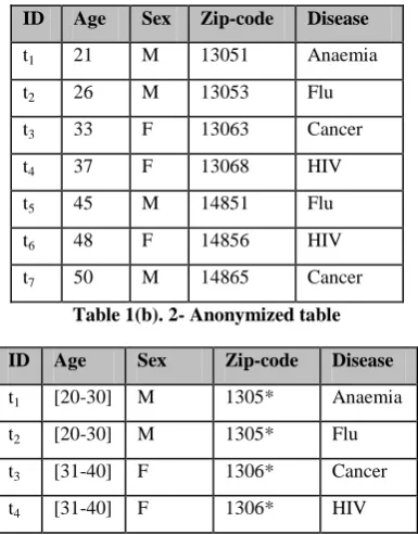
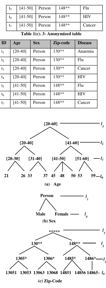
The traditional approach is to de-identify the microdata by removing identifying attributes such as name, SSN etc. [1]. Sweeney discovered that when the medical data was linked to the external voters list, 87% of the US citizens were identified [3]. This type of attack is coined as linking attack. To limit these kinds of attacks Sweeney proposed k-anonymity model where the domain of each quasi identifier attribute is divided into set of equivalence classes and each equivalence class contains at least k elements with the same value [2, 3]. In this model the quasi identifier attributes are suppressed or generalized. The data is generalized by constructing the Domain Generalization Hierarchies (DGH) for the corresponding quasi identifiers. For instance the DGH for age, gender and zip-code are shown in Fig 1(a), 1(b), 1(c) respectively. For the original Table 1(a), a 2-anonymised table is shown in Table 1(b) and 3-anonymized view is shown in Table 1(c). Here sensitive attributes are retained without any change.
Table 1(a). Original Table
ID Age Sex Zip-code Disease
t1 21 M 13051 Anaemia
t2 26 M 13053 Flu
t3 33 F 13063 Cancer
t4 37 F 13068 HIV
t5 45 M 14851 Flu
t6 48 F 14856 HIV
t7 50 M 14865 Cancer
Table 1(b). 2- Anonymized table
ID Age Sex Zip-code Disease
t1 [20-30] M 1305* Anaemia
t2 [20-30] M 1305* Flu
t3 [31-40] F 1306* Cancer
[image:1.595.333.526.510.757.2]t5 [41-50] Person 148** Flu t6 [41-50] Person 148** HIV t7 [41-50] Person 148** Cancer
Table 1(c). 3- Anonymized table
ID Age Sex Zip-code Disease
t1 [20-40] Person 130** Anaemia t2 [20-40] Person 130** Flu t3 [20-40] Person 130** Cancer t4 [20-40] Person 130** HIV t5 [41-50] Person 148** Flu t6 [41-50] Person 148** HIV t7 [41-50] Person 148** Cancer
In this paper we proposed minimum spanning tree based technique to achieve k-anonymity. In this approach the minimum spanning tree is constructed by considering quasi identifiers as the vertices of the spanning tree and the edges of the spanning tree represents hierarchical distance between two tuples. Initially, MST forest is constructed for the given microdata. We then remove all inconsistent edges which result in forming sub-trees. This process is repeated until each
subtree has k data points. Once this is achieved we generalize the data points adhering to k-anonymity for publishing. The rest of the paper is organised as follows: Section 2 surveys the related work. Section 3 presents an overview of minimum spanning tree. In Section 4 we present some formal definitions that were used in this paper. MST based anonymisation model in explained in section 5. Section 6 presents algorithms and discusses the complexity measures of our approach. The essential quality measures necessary for assessing our method are given in section 7. Section 8 show experimental evaluations to show the quality of our apporach and finally we conclude and present,possible future work in section 9.
2.
RELATED WORK
Sweeney and Samarati introduced k-anonymity, in which the domain of each quasi identifier attribute is partitioned into set of intervals by replacing the attribute values with corresponding intervals [2, 17]. Here, the tuple in the published table is indistinguishable from at least k-1 other tuples with respect to their quasi identifiers. Various models like global recoding, local recoding, multidimensional recoding, micro aggregation and clustering were proposed to achieve k-anonymity principle [14, 12, 6, 11]. In global recoding, all the attribute values in generalized table are obtained from the same level of domain hierarchy [20]. The advantage of the global recoding is that anonymized data can be viewed uniformly [19]. However, the anonymized dataset suffers from more information loss. In local recoding, the attribute values of generalized table are generalized to different levels in domain hierarchy. Multi-dimensional k-anonymity model assumes a d-dimensional domain space, which is divided into set of regions where each region contains at least k objects.
Another approach to accomplish k-anonymity is micro aggregation [18, 11]. Micro aggregation can be viewed as clustering problem where the size of the cluster is a constraint. Hua Zhuand Xiaojun showed k-anonymity as density based clustering problem in which set of tuples are grouped based on k-nearest-neighboring distance [5]. GaganAgarwal et.al proposed a method called anonymity via clustering [6]. In this method, initially quasi identifier records are clustered and then cluster centers are published. They considered r- GATHER as a metric to form clusters. A frame work called KACA to accomplish the k-anonymity in which grouping of the tuples is done based on attribute hierarchical structures [4]. A non-homogenous generalization for partitioning the data was also proposed that adheres to k-anonymity principle [19]. They enhanced this algorithm by proposing a randomized algorithm such that it does not compromise the attacker even if the algorithm is known [23].
A practically feasible algorithm called enhanced k-anonymity was proposed [12]. Their algorithm is based on full domain generalization approach. Fung et al. proposed classification model to protect the individual privacy [13]. They use top-down approach to achieve the anonymity constraint. Their model supports both numerical and categorical data. Graham et al. proposed bipartite graph model to anonymized the data using (k, l) grouping strategy thereby minimizing the adversary attacks [25,9].
[image:2.595.57.271.62.639.2]21 26 33 37 45 48 50 53 59 [20-30] [31-40] [41-50] [51-60]
[20-40] [41-60]
[20-60]
l2
l1
l0
l
3
(a) Age
Person
Male Female
l
1
l
0
1305* 1306* 1485* 1486*
130** 148**
*****
l
3l
2
l
1
(c) Zip-Code
Fig 1: Domain generalization hierarchies
13051 13053 13063 13068 14851 14856 14865- l0
3.
MINIMUM SPANNING TREE
PARTITIONING
Given a connected, weighted, undirected graph G = (V, E) together with a weight function 𝑐: 𝐸 → ℜ , where V is the set of vertices and E is the set of edges between the pair of vertices and c (e) specifying the weight of each edge. A spanning tree of G is a sub-graph which is a tree that connects all the vertices in G without having any cycles. The weight of a spanning tree is the sum of the weights of edges in that spanning tree. A minimum spanning tree (MST) of G is a spanning tree whose weight is less than or equal to weight of every other spanning tree of G. Well known algorithms for finding MST are Kruskal‟s algorithm [21], Borůvka‟s algorithm [26], and Prim‟s algorithm [22].
.
(a)
Data points(b)
MST forest
[image:3.595.56.250.236.678.2](c) Sub-trees of MST forest
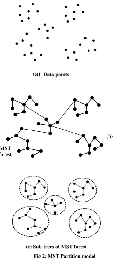
Fig 2: MST Partition model
For example, in Fig 2(a) sample data points are considered as the nodes of the graph and distances between these data points are edges of graph. By using the Kruskal algorithm we construct MST forest from the graph. Fig 2(b) show the MST forest for the given data points. After MST is constructed we remove the inconsistent edges from MST. Inconsistent edges are defined as those edges whose edge distances are significantly larger than average distance of the nearby edges
of MST. Hence the MST forest is partitioned into set of sub-trees as shown in Fig 2(c). The data points in each partitioned sub-tree are close to each other.
4.
PRELIMINARIES
The basic concepts and terminology used in the paper are discussed in this section. Let T be the microdata table that needs to be published. The table contains collection of tuples from domain D = I ×QI × SA, where I be the identifying attributes, QI be the quasi identifiers and SA be the sensitive attributes. For each tuple t ϵ T, the attribute value is denoted as t [A].
Definition 1 (Generalization) Let Ai be QID attribute and 𝐷𝐴𝑖 be the domain of Ai. Suppose 𝑑𝐴𝑖∈ 𝐷𝐴𝑖 is an instance of the attribute Ai is said to be generalized to 𝑑𝐴(𝑙)𝑖 if and only if there exists a binary relation ≼𝐴
𝑖
𝑓𝑖(𝑙)
such that 𝑑𝐴(0)𝑖 ≼𝐴 𝑖
𝑓𝑖(𝑙)
𝑑𝐴(𝑙)𝑖 , where f(l) is lth level of generalization over hierarchy tree and 𝑑𝐴(𝑙)𝑖 is lth level generalized value of 𝑑
𝐴𝑖. i.e 𝐷𝐴(𝑙)𝑖 = {𝑑𝐴(𝑙)𝑖|𝑑𝐴 𝑘 𝑖 ≼𝐴𝑓𝑖𝑖 𝑙 𝑑
𝐴𝑖
𝑙 , ∀𝑑
𝐴𝑖∈ 𝐷𝐴𝑖, 𝑘 = 0,1,2 … 𝑙 − 1}
Definition 2 (k-anonymity) The table is said to be k-anonymous if every combination of quasi identifier attribute values in a generalized table occurs k or more times.
5.
FRAMEWORK FOR MSTK
[image:3.595.338.524.430.722.2]The proposed framework minimum spanning tree partitioning (MSTK) is shown in Fig 3. This framework consists the following phases:
Step 1: Data Pre-processing and corresponding domain generalization hierarchies are created.
Step 2: Computing the hierarchical distances among data Points of given micro table to Generate distance matrix.
Step 3: Constructing the minimum spanning tree based on the distance matrix.
Step 4: Remove inconsistent edges from MST and form basic equivalence classes.
Step 5: Checking for anonymity of each equivalence class.
5.1
Data pre-processing
In this step the quasi identifiers attributes which are to be anonymized and their concept hierarchies are selected. For example Sex, Age and Zip-code attributes are quasi identifier attributes in the Table. 1 (a) and their domain hierarchies are shown in Fig 1.
5.2
Computing hierarchical distance
matrix
In this section we compute the distance matrix among all the tuple by using the following definitions
Definition 3 (Generalization Hierarchical Distance (GHD)): Let v and v1 be the two nodes of attribute generalization hierarchy and H be the height of the tree. The generalization hierarchical distance between the two node are defined as
𝐺𝐻𝐷 𝑣, 𝑣′ = 𝑣 − 𝑣′
𝐻 (1)
For example the values of an attribute Zip-code in hierarchy are {13051, 1305*, 130**, *****} as shown in Fig.1(c). Distance between 13051 and 130** is 2/3.The GHD is zero if both values are at same level or at the same leaf nodes and GHD is one if the value lies at the root
.
Definition 4 (Generalization Effort (GE)): Let t and t1be the tuple and generalized tuple respectively. The generalization effort of a tuple is defined as the amount of effort needed to change the attribute values of tuple one (low) level to another (generalized) level in domain generalization hierarchies of attributes of a tuple. i.e.
𝐺𝐸 𝑡, 𝑡′ = 𝐺𝐻𝐷 𝑎
𝑖, 𝑎𝑖′ (2) 𝑚
𝑖=1
Here, 𝑎𝑖, 𝑎𝑖′ are the original attributes values and generalized
attribute values of the tuple t respectively. For example, consider tuple t2 = {26, M, 13053} in the Table 1(a) and its generalized values 𝑡2′ = {[20-30], M, 1305*} in Table 1(b).
The GHD (26, [20 - 30]) = 0.333, GHD (M, M) = 0 and GHD (13053, 1350*) = 0.333, therefore 𝐺𝐸 𝑡2, 𝑡2′ = 0.666.
Definition 5 (Hierarchical Distance between two tuples):
Let t1 and t2 be the two tuples and t12 is the closest common generalization of tuples t1 and t2. The hierarchical distance between two tuples is defined as follows.
𝐻𝐷𝑖𝑠𝑡 𝑡1, 𝑡2 = 𝐺𝐸 𝑡1, 𝑡12 + 𝐺𝐸 𝑡2, 𝑡12 (3)
For example, consider two tuples the tuples t1 = {21, Male, 13051} and t2 = {26, Male, 13053} in the Table 3.1 (a) and their closest common generalization attribute values of tuples are t12 ={[20-30], M, 1305*}, which is obtained from the generalization attribute hierarchies of age, Sex and Zip-code as shown in Fig. 1 (a), (b), (c). Therefore the Hierarchical distance between two tuples is 1.333.
Definition 6 (Dissimilar Distance Matrix of Table): Given microdata T with n tuples {t1, t2, ..., tn} and each tuple contain m quasi-identifiers, The distance matrix is defined as follows and the distance matrix shown in Table 2:
[image:4.595.325.529.267.388.2]𝐷𝑇= 𝐻𝑑𝑖𝑠𝑡(𝑡𝑖, 𝑡𝑗 ) 𝑛×𝑛∀𝑖, 𝑗 ∈ 𝑛 (4)
Table 2. Distance Matrix
0 − − − − − −
1.333 0 − − − − −
4.667 4.667 0 − − − −
4.667 4.667 1.333 0 − − −
4.000 4.000 6.000 6.000 0 − −
6.000 6.000 4.000 4.000 3.333 0 −
4.000 4.000 6.000 6.000 2.000 4.000 0
5.3
Minimum Spanning Tree Forest
Construction
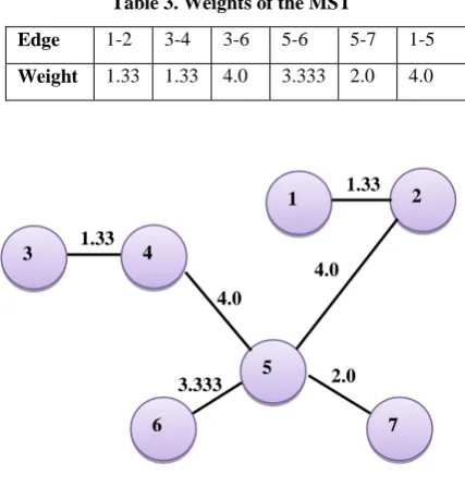
[image:4.595.322.536.524.748.2]After computing the distance matrix, MST is created by using above distance matrix. The nodes of the MST are the data points (records) of the micro table and the weight of edges are the concept hierarchical distance between two data points. We adopt Kruskal algorithm for constructing the MST. For example, the MST for the Table 1(a) is shown in Fig 4. and the corresponding weights are given in Table 3.
Table 3. Weights of the MST
Edge 1-2 3-4 3-6 5-6 5-7 1-5
Weight 1.33 1.33 4.0 3.333 2.0 4.0
Fig 4: MST forest
2
4 3
5
6 7
1
1.33
4.0 4.0
3.333 2.0
5.4
Pruning of inconsistence Edges from
MST Forest
For partitioning the MST, the inconsistent (longest) edges are pruned. This pruning process is performed based on inflection point. Finding the inflection point of the data is given as follows:
Inflexion point of the data: Let f be real values function i.e. f: 𝒟 → ℜ where ℜ is the set of real values and 𝒟 is the domain of f. Inflexion points are the points at which the concavity changes. Concave up corresponds to positive second derivative of the curve f, whereas Concave down corresponds to negative second derivative. So, the point at which the second derivative is equal to zero turns the concavity up to down and vice versa. Therefore at inflexion point, the curves‟ second derivative is equal to zero, i.e., 𝑓′′ = 0
If we consider the weights of the edges of a spanning tree to be a value of a random variable 𝒳. We assume that the weights of the spanning tree are normally distributed (𝒳 ~ N(ŵ,σ)), where ŵ be the mean and σ be the standard deviation. If f (x) is probability distribution function 𝒳, then f(x) satisfies the following.
Concavity: Let f be a real valued function over 𝑋, 𝑓: 𝑋 → ℜ is said to concave if ∀ 𝑥1, 𝑥2∈ 𝑋 𝑎𝑛𝑑 𝜆 ∈ 0, 1 , 𝑓 (1 − 𝜆 ∗
𝑥1+ 𝜆 ∗ 𝑥2) ≥ (1 − 𝜆 ) ∗ 𝑓(𝑥1) + 𝜆 ∗ 𝑓(𝑥2). 𝐼𝑓 f is twice
differentiable and second derivative is non-positive over X then f is concave i.e . 𝑓′′ 𝑥 ≤ 0, ∀𝑥 ∈ 𝑋 .
Convexity: Let f be a real valued function over 𝑋, 𝑓: 𝑋 → ℜ
is said to convex if ∀ 𝑥1, 𝑥2∈ 𝑋 𝑎𝑛𝑑 𝜆 ∈ 0, 1 , 𝑓 (1 − 𝜆 ∗
𝑥1+ 𝜆 ∗ 𝑥2) ≤ (1 − 𝜆 ) ∗ 𝑓(𝑥1) + 𝜆 ∗ 𝑓(𝑥2) . If f is twice
differentiable and second derivative is nonnegative over X then f is convex i.e 𝑓′′ 𝑥 ≥ 0, ∀𝑥 ∈ 𝑋.
Infection Point: The inflexion point of any real valued function over X, 𝑓: 𝑋 → ℜ is a point in X, at which the convexity switches to concavity vice versa.𝑖. 𝑒 the point 𝑥 ∈ 𝑋 such that 𝑓′′ 𝑥 = 0.
𝑓 𝑥 = 1
σ 2𝜋𝑒𝑥𝑝
−(𝑥 − ŵ)2
2𝜎2 ∀𝑥 ∈ ℜ
log 𝑓 𝑥 = −log(𝜎 2𝜋) − (𝑥 − ŵ)
2
2𝜎2
𝑓′ 𝑥 =− 𝑥 − ŵ
𝜎2 𝑓 𝑥
𝑓
′′𝑥 =
− 𝑥−ŵ 𝑓′ 𝑥 +𝑓 𝑥𝜎2
At the inflexion point 𝑓′′ 𝑥 = 0, then we have
𝑥 − ŵ 𝑓′ 𝑥 = 𝑓 𝑥
𝑥 − ŵ =𝑓𝑓(𝑥)′ 𝑥
𝑥 − ŵ 2= 𝜎2
𝑥 = ŵ ± 𝜎
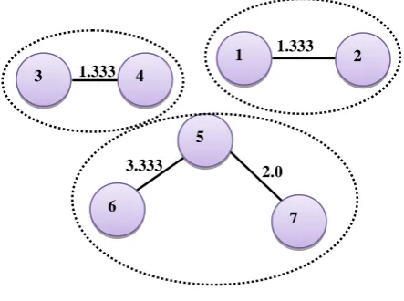
For the Fig.4, Mean and standard deviation of the weights are 2.665 and 1.265 respectively and hence the inflexion point of the MST is 2.665 + 1.265 = 3.9315. The edges which are greater than inflexion are pruned from MST. In the Fig.5, the values of the edges 4-5 and 1-5 are greater than 3.9315. So these edges are pruned from MST. This results into three disjoint sub-trees as shown in Fig. 6. Each sub-tree of forest represents as initial cluster (basic equivalence class) and the points in sub-tree are relatively close to each other.
Inducing the Equivalence classes: After splitting the MST forest into sub-trees, generalized equivalence class of each sub-tree are generated by using the attribute hierarchies. For example, in Fig 6, the QI values of sub-trees 1-2, 3-4 and 5-6-7 are {<21, M, 3051>, <26, M, 13053>}, {<33, F, 13063>, <37, F, 13068>}, {<45, M, 14851>, <48, F, 14856>, <50, M, 14865>} respectively and their generalized equivalence classes are <[20-30], M, 1305*>, <[30-40], F, 1306*>, <[40-50], Person, 148**>.
[image:5.595.322.537.295.435.2]Fig 5: Formation of Sub-trees from MST forest
Fig 6: Initial Basic Clusters
5.5 Checking for
k-
anonymity
In this section we discuss the anonymity parameter checking of each equivalence class, which are generated previously. For example if the required anonymity constraint is k= 2 for the Table 1(a), then it satisfied by the Table 1(b) formed by above step. That is each equivalence class contained at least two tuples which share the same value. If the anonymity constraint k=3 then Table 1(b) do not satisfied the anonymity constraint.
2 4
3
5
6
7 1 1.333
3.333 2.0
1.333
2
4 3
5
6
7 1
1.333
4.0 4.0
3.333
[image:5.595.315.537.486.651.2]So that the equivalence classes, whose size is less than k are merged based on the following distance metric.
Definition 7 (Distance between two equivalence classes):
Let C1 be an equivalence class containing n1 identical tuples t1 and C2 be an equivalence class containing n2 identical tuples t2. t12 is the closest common generalization of t1 and t2 the distance between two equivalence classes is defined as follows
𝐶𝐷𝑖𝑠𝑡 𝐶1, 𝐶2 = 𝑛1∗ 𝐻𝐷𝑖𝑠𝑡 𝑡1, 𝑡12 + 𝑛2∗ 𝐻𝐷𝑖𝑠𝑡 𝑡2, 𝑡12 (5)
[image:6.595.322.535.67.487.2]We considered the anonymity requirement as k=3 for the table 1(a). The generalized table as shown in table 1(b) does not satisfy the anonymity constraint. Hence, we need to merge these equivalence classes based on the distance metric to satisfy the anonymity requirement.
Table 4. Definitions
CreateMST (QI)
Generates an MST from microdata
EdgeSet (T) Returns the set of edges in minimum spanning tree T
AvgWeight (T)
Returns the average weight of edges in tree T
StdDev (T) Return standard deviation of weights of edges in tree T
PartMST (T, Ē)
Returns set of sub-trees after removing the inconsistence edges Ē from T. GenClass(st) Returns the generalized equivalence class
of each sub-tree (cluster).
6.
ALGORITHM
Our algorithm runs in two phases. During the first phase MST is constructed over the given microdata using Kruskal algorithm [21]. After constructing MST all the inconsistence edges are removed.
Algorithm 2: Minimum Spanning Tree based k-anonymity(MSTK)
Input: Quasi Identifier tuples, Attribute Hierarchies and k
Output: Set of equivalence classes
Method:
1. Begin
2. 𝑇 ← 𝐶𝑟𝑒𝑎𝑡𝑒𝑀𝑆𝑇(𝑄𝐼)
3. 𝐸 ← 𝐸𝑑𝑔𝑒𝑆𝑒𝑡 (𝑇) // Set of edges of MST 4. Ē = 𝛷
5. ŵ ← 𝐴𝑣𝑔𝑊𝑒𝑖𝑔𝑡 (𝑇)
7. 𝝈 ← 𝑺𝒕𝒅𝑫𝒆𝒗 (𝑻)
8. for each edge 𝒆 ∈ 𝑬 do
9. if (𝑾𝒆𝒊𝒈𝒉𝒕 𝒆 > ŵ + 𝝈) then
10. Ē ← Ē ∪ { 𝒆}
11. end if
12. end for
13. 𝑺𝑻 ← 𝑷𝒂𝒓𝒕𝑴𝑺𝑻 (𝑻, Ē)
13.. G ← Φ
14. G1← Φ 15. G2← Φ
16. for each sub-tree 𝑠𝑡 ∈ 𝑆𝑇 do
17. if 𝑠𝑡 > 𝑘 𝑎𝑛𝑑 𝑠𝑡 ≤ 2𝑘 − 1
18. 𝐺 ← 𝐺 ∪ 𝐺𝑒𝑛𝐶𝑙𝑎𝑠𝑠(𝑠𝑡) 19. else if ( 𝑠𝑡 > 2𝑘 − 1 ) do
20. call 𝑃𝑎𝑟𝑡𝑀𝑆𝑇 ( 𝑠𝑡, 𝑒 ) 21. else if ( 𝑠𝑡 < 𝑘)
22. 𝐺1= 𝐺1∪ 𝐺𝑒𝑛𝐶𝑙𝑎𝑠𝑠(𝑠𝑡)
23. end for
24. for each 𝐺1𝑖, 𝐺1𝑗 𝑖𝑛 𝐺1 𝑎𝑛𝑑 𝑖 ≠ 𝑗 do
25. 𝐺2= 𝐺2∪ 𝑚𝑒𝑟𝑔𝑒 𝐺1𝑖, 𝐺1𝑗
// 𝐺1𝑖, 𝐺1𝑗 have minimum distance
26. 𝐺1= 𝐺1− {𝐺1𝑖, 𝐺1𝑗}
27. end for
29. return (G + G2) // return k-anonymized table. 30. end Begin
In the second phase equivalence classes are generated and then the anonymity requirement is verified for each equivalence class. We defined various functions used in our algorithmic description of MSTK as shown in Table 4. The quasi identifier point set (QI) and anonymity constraint k is the input to the algorithm. Initially we create MST tree (T) on quasi identifiers QI. The nodes of MST are QI tuples and weights are the distance between two tuples. After construction of MST, the tree T is partitioned by removing all edges whose weight 𝑤 > 𝐴𝑣𝑔𝑊𝑒𝑖𝑔𝑡 𝑇 + 𝑆𝑡𝑑𝐷𝑒𝑣 𝑇 . This results into set of sub-trees ST = {ST1, ST2,...} each representing an equivalence class. Let 𝑇′ be the MST forest,
obtained after removing inconsistent edges, i.e., 𝑇′= 𝑆𝑇 𝑖 𝑖
and 𝑆𝑇𝑖 𝑖= ∅ where 𝑆𝑇𝑖, ∀𝑖 is a sub-tree of the forest (step
Case 1: If the numbers of data points in the sub-tree lie between the k and 2k-1, then it satisfies the k-anonymity property(line 17-18). Now, GenClass(STi) is called to substitute appropriate domain ranges to all the data points of the subtree using attribute domain generalization hierarchies.
Case 2: If the number of data points in the sub-tree are greater than 2k-1 , recursively we remove the inconsistent edges from the subtree until k-anonymity property is satisfied(line 19-20 ). We then generalize the data points by calling GenClass.
Case 3: If the number of data points in subtree are less than k, we generalize the data points in the subtree to form equivalence classes. In order to achieve k-anonymity, we merge the equivalence classes by calculating the pair wise distances between the equivalence classes (lines 24-27).
6.1 Complexity Analysis
The complexity for computing the distance matrix is 𝑂 𝑛2 and to construct the MST from n number of data points is 𝑛 𝑙𝑜𝑔2𝑛. The maximum number of inconsistent edges that can
be removed from MST forest are n-1, hence the time required for removing the inconsistent edges and to form sub-trees (equivalence class) is 𝑂 𝑛 . Let C (𝐶 ≪ 𝑛) be the total number of equivalence classes formed by after removing the inconsistent edges. Then the time complexity to check anonymity of each equivalence class is 𝑂 𝐶 . Therefore, the total time needed for executing the algorithm is 𝑂 𝑛2 + 𝑂 𝑛 𝑙𝑜𝑔2 𝑛 + 𝑂 𝑛 + 𝑂 𝐶 ≈ 𝑂 𝑛2 .
7.
QUALITY MEASURES OF
ANONYMIZATION
Protecting privacy of the data is achieved through anonymization. The other aspect of privacy is to produce the anonymized data that must be useful for deriving useful patterns for statistical analysis i.e., published data should remain for practical use. There are broad categories of information metrics for measuring the data usefulness. A data metric measures the data quality of the entire anonymous table with respect to the data quality in the original table. A quality metric guides each step of an anonymization (search) algorithm to identify an anonymous table with maximum utility or minimum information loss. However, some data publishers concentrate on anonymization process and some on utility of the data. To overcome this trade-off scenario the anonymized table is measured with reasonable information metrics to measure “similarity” between the original data and the anonymous data. This underpins the principle of minimal distortion. Several quality measure such as minimal distortion [3, 17], Information loss [26, 08], Discernibility metric [10], classification metric [27], information trade-off metric (entropy) [13], model accuracy and query quality [14] and normalized equivalence class metric [10] were widely used in the literature. These metrics are used based on anonymization problem. In this paper we used information loss, Discernibility and Normalized average equivalence class for measuring the quality of anonymize table.
7.1 Information Loss
Information loss is data metric proposed by Gabriel [8] to capture the information loss by generalizing a specific value to a generalized value. The information loss is computed based on attribute domain hierarchies. Information losses for both numerical and categorical attributes are given in equations 6 and 7 respectively.
𝐼𝐿𝑛𝑢𝑚𝑒𝑟𝑖𝑐𝑎𝑙 = (𝑈(𝑈 − 𝐿)𝑖− 𝐿𝑖) (6)
Here, [Ui, Li] be the upper and lower boundary values of the specific equivalence class and [U, L] be the upper and lower values of entire domain range satisfying the relation 𝑈𝑖, 𝐿𝑖 ⊆
[𝑈, 𝐿].
𝐼𝐿𝑐𝑎𝑡𝑒𝑔𝑜𝑟𝑖𝑐𝑎𝑙 = (𝐿𝑣𝐿− 1) (7)
Here, Lv is the number of nodes rooted from the current node
and L is number of leaf nodes of the domain hierarchy. If the tuple consists of „m‟ numerical attributes and „n‟ categorical attributes then the information loss of the whole tuple is
𝐼𝐿𝑡𝑢𝑝𝑙𝑒 = 𝐼𝐿(𝑛𝑢𝑚𝑒𝑟𝑖𝑐𝑎𝑙 )𝑖
𝑚
𝑖=1
+ 𝐼𝐿(𝑐𝑎𝑡𝑒𝑔𝑜𝑟𝑖𝑐𝑎𝑙 )𝑖
𝑛
𝑖=1
(8)
The total information loss for the anonymized table T is 𝐼𝐿𝑇=
𝑛𝑖∗ 𝐼𝐿𝑡𝑢𝑝𝑙𝑒 𝑘
𝑖=1
𝑛𝑖 𝑘 𝑖=1
(9)
7.2 Discernability
The discernibility metric (DM) [7, 10] addresses the notion of loss by charging a penalty to each record for being indistinguishable from other records with respect to quasi identifier group (equivalence class). If a record belongs to a quasi-identifier group of size |E|, then penalty for the record will be |E|. The overall penalty cost of generalized table T is given by
𝐷𝑀 =
𝐸
2𝐸𝑞𝑢𝑖𝑣𝑎𝑙𝑒𝑛𝑐𝑒 𝑐𝑙𝑎𝑠𝑠𝑒𝑠 𝐸
(10)
The objective of anonymization is to minimizing discernibility cost. For example, in the anonymized table of our running example Table 1(b) contain three equivalence classes {<[20-30], M, 1305*>, <[30-40], F, 1306*>, <[40-50], Person, 148**>} and their group sizes are 2, 2, 3 respectively. The discernibility of the table is 22 + 22 + 32 = 17.
7.3 Normalized Average Equivalence Class
The intuition of this metric is to measure how well the partitioning approaches the best case when each tuple is generalized in a group of k indistinguishable tuples. i.e.,
𝐶𝐴𝑉𝐺 = 𝑡𝑜𝑡𝑎𝑙 𝑛𝑢𝑚𝑏𝑒𝑟 𝑜𝑓 𝑟𝑒𝑐𝑜𝑟𝑑𝑠
𝑡𝑜𝑡𝑎𝑙 𝑛𝑢𝑚𝑏𝑒𝑟 𝑜𝑓 𝑒𝑞𝑢𝑖𝑣𝑎𝑙𝑒𝑛𝑐𝑒 𝑐𝑙𝑎𝑠𝑠𝑒𝑠 ∗ 𝑘 (11)
The objective of anonymization is to reduce the normalized average equivalence class size. If CAVG is low, more number of equivalence classes will be generated and hence we can achieve better anonymization.
8. EXPERIMENTAL RESULTS
experimentation. The size of the dataset was 30,162 tuples after removing tuples with missing values
Table 5. Adult Dataset Description
Attribute Type Distinct
values
Tree height
1 Age Numeric 74 4
2 Work class Categorical 7 3
3 Gender Categorical 2 1
4 Education Categorical 16 4
5 Race Categorical 5 2
6 Occupation Categorical 14 2
We considered the projection of the Adult dataset with six attributes Age, Work Class, Gender, Education, Race and Occupation. The corresponding tree heights of the chosen attributes and their type and number of distinct values are shown in the Table 3.
The proposed method is compared with a global recoding method basic Incognito [20]. Comparison is done based on different quality metrics like information loss, discernability metric and normalised average equivalence class size. Experiments are shown in Fig 6(a), Fig 6(b) and Fig 6(c). Fig 6(a) shows the information loss when the value of k-increases for both incognito and our approach. Our method shows a significant improvement by reducing the information loss when compared to incognito.
Fig 6(b) shows how discernability metric (DM) differs for both incognito and MSTK. For DM value, out of 7 experiments (k=3…21) with step size of k=3, MSTK outperforms Incognito. We found that, our approach achieves better discernability.
Fig 6(c) shows that our approach achieves better normalized average equivalence class than incognito. For lower value of k the incognito‟s Normalised average equivalence class size (CAVG) is very high where as in our minimum spanning tree based k-anonymity (MSTK) approach the CAVG is quite low for any value of k. The running time complexity however is more for our approach but a promising quality is achieved when compared with incognito. We can decrease the time by using parallel algorithms for construct the minimum spanning tree.
Fig 6(a): Information Loss
Fig 6(b): Discernability
Fig 6(c): Normalized Average Equivalence Class
Fig 6: Performance of Different Methods with Variant k
9.
CONCLUSION AND FUTURE WORK
In this paper, we studied the problem of minimum spanning tree based technique to achieve k-anonymity. We compared our approach with incognito technique based on quality metrics like information loss, CAVG and discernability. Our technique showed a significant improvement when compared with incognito. The complexity of our algorithm is O (n2). The experimentation clearly signifies the quality that can be achieved using our approach. In future we would like to enhance our MSTK method by adopting parallelism to construct the MST and thereby reducing the running time.
10.
REFERENCES
[1] Agrawal, R., and Srikant, R. 2000. Privacy preserving data mining, In Proceedings of the ACM SIGMOD International Conference on Management of Data, Dallas, Texas, pp. 439- 450.
[2] Sweeney, L. 2002. k-anonymity: a model for protecting privacy, International Journal on Uncertainty, Vol.10(5), pp.557–570.
[3] Sweeney, L. 2002. Achieving k-anonymity privacy protection using generalization and Suppression, International Journal on Uncertainty, Fuzziness and Knowledge-based Systems, Vol. 10(5), pp 571–588. [4] Jiuyong, Li., Raymond Chi-Wing, W., Ada Wai-Chee Fu
and Jian Pei. 2006. Achieving k-Anonymity by clustering in Attribute Hierarchical Structures, In Proceeding of the 8th International Conference on Data Warehousing and Knowledge Discovery, Krakow, Poland, pp.405-416. [5] Hua Zhu and XiaojunYe. 2007. Achieving k-anonymity
[image:8.595.325.536.71.195.2] [image:8.595.60.277.576.687.2]the 8th International conference on Web-age information management conference (WAIM'07), pp. 745 -752. [6] Agrawal, G., Feder, T., Krishnaram, K., Samir, K., Rina
Panigrahy, Dilys, T., and Zhu. 2006. Achieving Anonymity via clustering PODS‟06, Chicago, Illinois, USA.
[7] Roberto,J., Bayardo and Agrawal,R. 2005. Data Privacy Through Optimal k-Anonymisation, In Proceeding Proceedings of the 21st International Conference on Data Engineering, pp.217-228
[8] Gabriel, G., Panagiotis, K., Panos, K., and Nikos, M. 2007. Fast Data Anonymisation with Low Information Loss, In Proceedings of the 33rd International conference on Very large databases(VLDB‟07), Vienna, Austria, pp. 758-769.
[9] Manolis, T., Nikos, M., and Panos Kalnis. 2010. Local and global recoding methods for anonymizing set-valued data, The VLDB Journal Vol. 20, pp.83–106.
[10] Jiuyong, Li., Wong, R.C.W., Fu, A.W.C., and Jian Pei. 2008. Anonymisation by Local Recoding in Data with Attribute Hierarchical Taxonomies, IEEE Transactions On Knowledge and Data Engineering, Vol. 20, pp.1181-1194.
[11] Michael, L., and Mukherjee, S. 2005. Minimum Spanning Tree Partitioning Algorithm for Micro-aggregation, IEEE Transactions on Knowledge and Data Engineering, Vol. 17, No. 7, pp. 902-911.
[12] LeFevre, K., David, J., DeWitt, and Ramakrishnan, R. 2005. Multidimensional k-anonymity, In Proceedings of the 22nd International Conference on Data Engineering (ICDE‟06), Washington, USA.
[13] Fung, B.C.M., Wang, K., and Yu, P.S. 2005. Top-down specialization for information and privacy preservation, In Proceedings of the ICDE‟05, pp.205–216.
[14] Xu, J.,Wang, W., Pei, J.,Wang, X., Shi, B., and Fu, A.W.C. 2006. Utility-based anonymisation using local recoding, In Proceedings of the SIGKDD‟06, pp.785– 790.
[15] Vidya, J. and Clifton, C. 2003. Privacy preserving k-means clustering over vertically partitioned data, In Proceedings of the 9th ACM SIGKDD International conference on Knowledge discovery and data mining, Washington, USA, pp. 206-215.
[16] Wright, R. and Yung, Z. 2004. Privacy preserving Bayesian network structure computation on distributed heterogeneous data, In Proceedings of the KDD‟04, Seattle, WA, USA, pp.713-718.
[17] Samarati, P. 2001. Protecting respondent‟s identities in microdata Release, In IEEE Transactions on Knowledge and Data Engineering, Vol.13 (6). pp. 1010-1027 [18] Domingo-Ferrer, J. and Torra, V. 2005. Ordinal,
continuous and heterogeneous k-anonymity through micro-aggregation, ACM transactions on Data Mining and Knowledge Discovery, vol. 11(2), pp.195-212. [19] Wong, W.K., Nikos Mamoulis and Cheung, W. D. 2010.
Non-homogeneous Generalization in Privacy Preserving data Publishing, In Proceedings of the SIGMOD‟10, Indianapolis, Indiana, USA, pp. 747-758.
[20] LeFevre, K., DeWitt, D.J., and Ramakrishnan, R. 2005. Incognito: Efficient Full-domain k-Anonymity, In Proceedings of the ACM SIGMOD, Baltimore, Maryland, USA, pp 49–60.
[21] Kruskal, J. 1956. On the shortest spanning sub tree and the travelling sales problem. In Proceedings of the American Mathematical Society, pp. 48-50.
[22] Prim, R. 1957. Shortest connection networks and some generalization, In Bell systems technical journal, pp.1389-1401.
[23] LeFevre, K.D., DeWitt, J. and Ramakrishnan, R. 2006. Workload-aware Anonymization, In Proceedings of the KDD‟06, PA, USA, pp. 277–286.
[24] Newman, D.J., Hettich, S., Blake, C.L., and Merz, C.J. 1998. UCI Repository of Machine Learning databases, http://www.ics.uci.edu/~mlearn/MLRepository.html [25] Graham, C., Srivastava, D. 2011. Ting Yu and Qing
Zhang, Anonymizing Bipartite graph data using safe groupings, VLDB journal, pp. 115-139.
[26] Elisa, B., Beng Chin O., Yang, Y., and Deng, R.H. 2005.Privacy and Ownership Preserving of Outsourced Medical Data, In Proceedings of the IEEE International Conference on Data Engineering, pp. 521-532.