Combined Artificial Neural Network Model for Estimation
of Pressure Drop for Flow of CMC and Soil in Aqueous
Solution
Shekhar Pandharipande
Associate Professor, Dept. of Chemical Engineering,Laxminarayan Institute of Technology, RTM Nagpur University,
Nagpur, India
Rachana S. Ranshoor
M.Tech Third Semester, Laxminarayan Institute of Technology, Nagpur, IndiaABSTRACT
Estimation of pressure drop for flow of Non -Newtonian fluid is a common situation & conventional models fail to address it with high accuracy & are to be system specific. Present work is aimed to explore the possible use of the Artificial Neural Network in developing combined models for the estimation of pressure drop as a function of flowrate, density, & concentration of CMC & soil in water mixture in a pipeline. Experimental runs are conducted & the 81 data points generated are divided into 64 & 17 as training & test data points respectively. The RMSE values for S1 & C1 models are 0.023 & 0.016 respectively. Further evaluation done by calculating & comparing the percentage relative error shows that, most of the predicted values have accuracy level of around 90% & is acceptable. The present work has successfully highlighted the potential of Artificial Neural Network in modeling complex processes.
General Terms
Artificial Neural NetworkKeywords
Artificial Neural Network, Soil-CMC-Water Solution, Pressure Drop Estimation, Non-Newtonian Fluid.
1.
INTRODUCTION
Industrial processes involve the handling of fluids of different features. Newtonian fluids are those which obey the Newton’s law of viscosity, which states that the shear stress is directly proportional to the rate of shear & the constant of proportionality is known as viscosity. Viscosity of Newtonian fluid is dependent on temperature however it is independent of applied shear rate & the graph plotted between the rate of shear & shear stress is a straight line passing through origin. Water, low weight pure hydrocarbons & their mixtures such as benzene, toluene, and xylene etc, several gases including air come under the Newtonian category. There are several other fluids which do not follow the Newton’s law of viscosity & the graph plotted between the shear stress & shear rate is not linear & may even be time dependent. Hence constant coefficient of viscosity can-not be defined. Slurries, oils, creams, shampoos, greases, paints, dairy products, polymer melts, sauces, ice creams, lubricating oils, drilling mud & many more fluids fall in this category of Non-Newtonian fluid. Fluid flow in close conduits, flow channels & pipe lines is common in several processes & designing of
There are several supporting equations or models suggested involving parameters such as Reynolds number, friction factors etc. Due to complex behavior of Non-Newtonian fluids, correlations & modeling equations have to be system specific & seldom found to be accurate.
CMC is readily soluble in water & depending upon the concentration of CMC in the aqueous solution, it may have Non-Newtonian behavior. CMC (Carboxymethyl cellulose) has wide applications in oil, textile, printing & dyeing, paper & ceramic industry etc [1]. It is one of the important raw materials used in tooth paste production, mixes liquid ingredients with solid materials & ensures that the tooth paste has good performance in molding, flow & posses appropriate viscosity.
In last few years, CMC were used as Non-Newtonian fluids by researchers for various studies. Shankar .P, Himanshu Vyas, Kalaichelvi .P and Muthamizhi .K [2] studied mixing characteristics of 0.5%CMC in double jet mixer. F.T.Pinho & J.H.Whitelaw [3] had well discussed about the delay in transition from laminar to turbulent flow caused by shear thinning, where experiments were carried out by using CMC. Determination of total head loss & friction factor corresponding to pressure drop & loss coefficient caused by fittings & valves, using CMC aqueous solution was studied by Adelson Balizario Leal [4] et al. Diego Gomez-Diaz & Jose M. Navaza [5] studied the apparent viscosity & the influence of shear rate on different polymer concentration in aqueous solution of CMC, & also the effect of temperature on rheological behavior, & found that the behavior parameter, n, decreased when CMC concentration increased. Bart C.H. Venneker [6] et al studied about the turbulent flow of shear thinning fluid in stirred tank. F.T.Pinho [7] et al, studied the pressure drop of shear thinning in laminar flow across a sudden expansion.
Soil or sediments in water is commonly seen in rivers, dams etc. Similar situation is also encountered during the exploration of crude from the oil well. The presence of soil in water makes it muddy & sticky. Thus system may possess Newtonian or Non-Newtonian behavior that is dependent upon the soil concentration. The flow of sediments involves significant pressure loss. Therefore it becomes difficult for the engineers, the accurate predictions of water resources parameters.
middle reach of the river Dijle. M. R. Mustafa, M. H. Isa, R. B. Rezaur developed the ANN model for the prediction of water resources parameters like sediment discharge, water discharge, rainfall, runoff & water quality.[9]
Artificial Neural Network is emerging as a modeling tool for processes involving complex non-linear multivariable correlation. There are several architectures of Artificial Neural Network & error back propagation (EBP) is common for modeling applications. Each layer has a number of processing elements called as neurons or nodes which is decided by the number of input & output parameters that are to be correlated. The number of hidden layers & the number of nodes present in each layer is decided by the complexity of the modeling problem involved, & may vary from algorithm to algorithm. Each node present in a layer is connected with every other node in the succeeding layer by means of a connectionist constants also called as weights. The output from a neuron is altered by the weight when it reaches to the nodes in succeeding layers. The summation of the product of all the input signals received by a neuron is transformed by sigmoid function & acts as an output signal for neurons in the next layer. Training of the EBP is essential & the algorithm suggested by Rummelhart [10] is popular. Artificial neural network has been applied in variety of situations for estimation, modeling, fault detection & diagnostic, optimization & control.
Several applications of ANN in modeling of various processes is reported in literature. Optimizing topology in developing artificial neural network model for estimation of hydrodynamics of packed column [12]. ANN is also used for the estimation of pressure drop of packed column [13]. ANN is used to detect leak in pipelines [14]. Artificial Neural Network has also been used by S.L. Pandharipande along with his co-workers for Modeling of Equilibrium Relationship for Partially Miscible Liquid-Liquid Ternary System [15] for Modeling of Packed Bed Using Artificial Neural Network [16], & also for Estimation of Composition of a Ternary Liquid Mixture with its Physical Properties such as Refractive Index, pH and Conductivity [17]
In present work an effort has been made to explore the possible use of the Artificial Neural Network in developing combined models for the estimation of pressure drop as a function of flowrate, density & concentration of CMC & soil in water mixture. The novel feature of the present work is incorporation of parameters like flow of pure water, aqueous solution of CMC, aqueous solution of soil & aqueous solution of both CMC & soil in a single combined model. Experimental runs are conducted for measurement of pressure drop for flow of various combinations & concentration of soil & CMC in water in a pipe line.
Two Artificial Neural Network models are developed & the predicted values of the output parameters are compared with the actual values obtained from experimentation.
2.
MATERIALS & METHODS
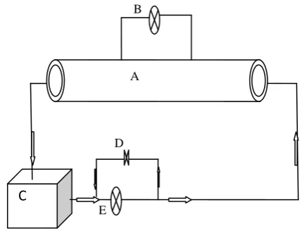
Figure 1 show the schematic of the experimental setup. It consists of a reservoir tank having 60 liters capacity, 1HP centrifugal pump & 9 feet long acrylic pipe having 25 mm diameter.
Experiments are performed by pumping these solutions into the pipe & noting head loss for varying flow rate conditions.
Experimental runs are conducted separately for different combinations of soil & CMC in water as given below: I. For CMC-Water solution
II. For soil-water solution III. For Soil-CMC-water solution
The various concentrations of CMC water solutions prepared for experimental runs are 0.192%, 0.29%, 0.392%, 0.492%, & 0.592% by wt.
Similarly soil water mixture concentrations are 1%,2%,3% by wt.
Concentration of soil & CMC in water mixture is 2% & 0.592% by wt respectively for combined system.
Head loss is measured by using an inverted manometer, whose limbs are 3 feet apart. Flow rate is measured by weighing the solution collected for known interval of time.
Pressure drop is calculated by using ∆P= h*ρ*g
B
A
D
[image:2.595.331.546.333.497.2]E
Fig 1: Schematic of the experimental setup
C→ storage tank; E→ centrifugal pump; A→ acrylic pipe of diameter 25mm;B→ inverted U tube manometer, whose limbs are 3 feet apart; D→ valve to control flowrate.
The details of the topology of the two ANN models S1 & C1 developed in the present work using elite-ANN© [11] is given in table 1.The experimental data generated is divided in two parts , one part containing 64 data points as training data set and the other with 17 data points as test data set.
Table 1. Neural network topology for ANN models
Name of ANN models
Numbers of neurons Data points RMSE Iterations
Input layer
1st hidden
layer
2nd hidden
layer
3rd hidden
layer
Output layer
Training data set
Test data set
Training data set
Test data set
S1 4 0 5 5 2 64 17 0.023 0.037 50000
C1 4 10 10 10 2 64 17 0.016 0.033 50000
The typical schematic of the architecture of ANN used in the present work is shown in figure number 2.
Input Layers Hidden Layers Output Layers
Velocity Head loss
Concentration
of soil
Concentration of CMC Pressure drop
[image:3.595.52.545.99.485.2]Density
Figure 2: Neural network architecture
3.
RESULT & DISCUSSIONS
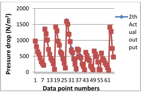
Figures 3 & 4 show the comparison of the actual & predicted values of head loss & pressure drop for training data set using ANN model S1.
Fig 3: Comparison of actual and predicted values of head loss for training data set using ANN model S1
Fig 4: Comparison of actual & predicted values of pressure drop for training data set using ANN model S1
Figures 5 & 6 show the comparison of actual & predicted values of head loss & pressure drop for test data set using ANN model S1.
Fig 5: Comparison of actual & predicted values of head loss for test data set using ANN model S1
0 5 10 15 20
1 6 11 16 21 26 31 36 41 46 51 56 61 66 1th Actual outpu t
Data point numbers
He
ad
Lo
ss
(
cm)
0 500 1000 1500 2000
1 7 13 19 25 31 37 43 49 55 61
2th Actu al outp ut
Pr
e
ss
u
re
d
ro
p
(
N
/m
2
)
Data point numbers
0 5 10 15
1 3 5 7 9 11 13 15 17 1th Actual output 1th Predicte d output
Data point numbers
He
ad
Lo
ss
(
[image:3.595.316.549.483.615.2]Fig 6: Comparison of actual & predicted values of pressure drop for test data set using ANN model S1
It is observed from these graphs that the predicted values are fairly close to the actual values.
[image:4.595.316.540.76.241.2]Figures 7 & 8 show the comparison of actual & predicted values of head loss & pressure drop for training data set using ANN model C1.Similarly figure 9 & 10 show the comparison of actual & predicted values of head loss & pressure drop for test data set using ANN model C1
.
Fig 7: Comparison of actual & predicted values of head loss for training data set using ANN model C1
[image:4.595.317.541.218.371.2]Fig 8: Comparison of actual & predicted values of pressure drop for training data set using ANN model C1
[image:4.595.58.279.349.472.2]Fig 9: Comparison of actual & predicted values of head loss for test data set using ANN model C1
Fig 10: Comparison of actual & predicted values of pressure drop for test data set using ANN model C1.
Graphs obtained for training & test data set by ANN model C1 also give fairly close predicted values for head loss & pressure drop to the actual values. Hence it is felt necessary to compare predicted values of S1 & C1.
Developed ANN models S1 & C1 are then compared for predicted values of head loss & pressure drop with actual values graphically in a combined manner. Figures 11 & 12 show these comparisons.
Fig 11: Comparison of actual & predicted values of head loss using ANN models S1 & C1
0 500 1000 1500
1 3 5 7 9 11 13 15 17 2th Actual output
Pr
es
su
re
d
ro
p
(
N
/m
2
)
Data point numbers
0 5 10 15 20
1 7 13 19 25 31 37 43 49 55 61
1th Actual outpu t
Data point numbers
He
ad
Lo
ss
(
cm)
0 500 1000 1500 2000
1 7 13 19 25 31 37 43 49 55 61
2th Act ual out put
Pr
e
ss
u
re
d
ro
p
(
N
/m
2
)
Data point numbers
0 5 10 15
1 3 5 7 9 11 13 15 17
1th Actual output
He
ad
Lo
ss
(
cm)
Data point numbers
0 500 1000 1500
1 3 5 7 9 11 13 15 17
2th Actual output
Data point numbers
Pr
es
su
re
d
ro
p
(
N
/m
2
)
0 5 10 15 20
1 7 13 19 25 31 37 43 49 55 61
1th Actu al outp ut
Data point numbers
He
ad
Lo
ss
(
[image:4.595.318.537.501.619.2] [image:4.595.56.282.512.659.2]Fig 12: Comparison of actual & predicted values of pressure drop using ANN models S1 & C1
The accuracy of prediction of ANN models S1 & C1 is further compared by estimating percentage relative error calculated as given below.
%E= [(Actual values - Predicted values)/Actual values]*100
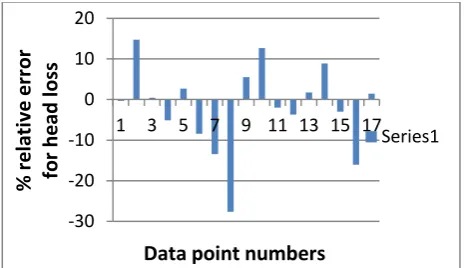
[image:5.595.316.549.71.205.2]Figures 13 & 14 show the percentage relative error for head loss & pressure drop for training data set using ANN model S1.
Fig 13: percentage relative error for head loss for training data set using ANN model S1.
Fig 14: percentage relative error for pressure loss for training data set using ANN model S1
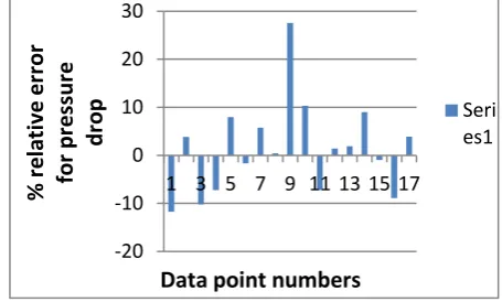
Figures 15 & 16 show the percentage relative error for head loss & pressure drop for test data set using ANN model S1.
[image:5.595.318.542.248.386.2]Fig 15: Percentage relative error for head loss for test data set using ANN model S1
Fig 16: Percentage relative error for pressure drop for test data set using ANN model S1
Figures 17 & 18 show the percentage relative error for head loss & pressure drop for training data set. Similarly figures 19 & 20 shows the percentage relative error for head loss & pressure drop using ANN model C1.
Fig 17: Percentage relative error for head loss for training data set using ANN model C1
0 500 1000 1500 2000
1 7 13 19 25 31 37 43 49 55 61
Actua l Press ure drop outp ut
Pr
es
su
re
d
ro
p
(
N
/m
2)
Data point numbers
-60 -40 -20 0 20 40
1 7 13 19 25 31 37 43 49 55 61 Series1
Data point numbers
%
re
la
ti
ve
e
rr
o
r
fo
r
h
e
ad
lo
ss
-60 -40 -20 0 20 401 7 13 19 25 31 37 43 49 55 61 Se…
%
rela
ti
ve
e
rr
o
r
fo
r
p
re
ss
u
re
d
ro
p
Data point numbers
-30 -20 -10 0 10 20
1 3 5 7 9 11 13 15 17 Series1
%
re
la
ti
ve
e
rr
o
r
fo
r
h
ea
d
lo
ss
Data point numbers
-40 -30 -20 -10 0 10 20
1 3 5 7 9 11 13 15 17 Series1
%
re
la
ti
ve
e
rr
o
r
fo
r
p
re
ss
u
re
d
ro
p
Data point numbers
-60 -40 -20 0 20
1 7 13 19 25 31 37 43 49 55 61
Series1
Data point numbers
[image:5.595.57.278.536.658.2]Fig 18: percentage relative error for pressure loss for training data set using ANN model C1
Fig 20: Percentage relative error for pressure drop for test data set using ANN model C1
Fig 19: Percentage relative error for head loss for test data set using ANN model C1
[image:6.595.313.541.73.210.2]The details of the distribution of % relative error for the data points for ANN model S1 & C1 is given in table 2
Table 2. Distribution of % relative error
Name of ANN model
Data points % Relative error =[ (Actual value –Predicted value)/ Actual value ]× 100 Parameters 0 to ±10 ±10 to ±20 >±20
S1 Training data points 64
Head loss 47 13 4
Pressure drop 48 12 4
Test data points 17
Head loss 12 4 1
Pressure drop 13 3 1
C1 Training data points 64
Head loss 52 9 3
Pressure drop 51 11 2
Test data points 17 Head loss 12 4 1
Pressure drop 13 3 1
-80 -60 -40 -20 0 20
1 7 13 19 25 31 37 43 49 55 61
Series1
%
re
la
ti
ve
e
rr
o
r
fo
r
p
re
ss
u
re
d
ro
p
Data point numbers
-20 -10 0 10 20 30 40
1 3 5 7 9 11 13 15 17 Serie s1
Data point numbers
%
re
la
ti
ve
e
rr
o
r
fo
r
h
ea
d
lo
ss
-20 -10 0 10 20 30
1 3 5 7 9 11 13 15 17 Seri es1
%
re
la
ti
ve
e
rr
o
r
fo
r
p
re
ss
u
re
d
ro
p
[image:6.595.65.532.460.698.2]4. CONCLUSION
The modeling of dynamics of Non-Newtonian fluid is a complex phenomenon & has so often posed challenges to engineers. The estimation of pressure drop for flow of Non -Newtonian fluid is a common situation. The conventional mathematical models do address to this situation, however with a lot of deviation & poor performance. These models need to be system specific & hence to be developed separately.
The present work has novel feature in developing combined model that estimates head loss & pressure drop for flow of fluids involving flow of pure water, aqueous solution containing soil, aqueous solution containing CMC & aqueous solution containing both CMC & soil. The 81 data points generated from experimental runs are divided into 64 & 17 as training & test data points respectively. The RMSE values for S1 & C1 models are 0.023 & 0.016 respectively for training data sets. Elaborative performance evaluation of both these models S1 & C1 is done by calculating & comparing the percentage relative error for all the data points which shows that , for most of the predicted values of head loss & pressure drop, the accuracy is around 90% & is acceptable. However the accuracy of prediction using model C1 is superior marginally when compared with model S1.
The present work is demonstrative & successfully highlighted the potential of Artificial Neural Network in modeling complex process. It is felt necessary to extend it to several other systems involving combinations of Newtonian & Non-Newtonian fluids.
5. ACKNOWLEDGMENT
Authors are thankful to Director, LIT, Nagpur for the facilities and encouragement provided.
6. REFERENCES
[1] R.P.Chabra “Non-Newtonian Fluids: An Introduction” [2] Shankar, P., Vyas, H., Kalaichelvi, P. & Muthamizhi, K.
2012. Experimental Analysis of Mixing Characteristics of Carboxymethyl Cellulose Solutions in a Doube Jet Mixer.
[3] Pinho, F.T. & Whitelaw, J.H. 1990. Flow of Non-Newtonian Fluid in Pipe.
[4] Leal, A.B., Calcada, L.A. & Scheid, C.M. 2nd Mercosur Congress On Chemical Engineering, 4th Mercosur Congress on Process Systems Engineering, Proceeding in ENPROMER.
[5] Diaz, D.G & Navaza, J.M. 2003. Rheology of Aqueous Solutions of food Addictives Effect of Concentration, Temperature & Blending.
[6] Venneker, B.C.H., Derksen, J.J, Van Den Ayyer, & Harry, E.A. 2010. Turbulent Flow of Shear Thinning Fluid in Strried Tank
[7] Pinho, F.T., Oliveira, P.J. & Miranda, J.P., 2003. Pressure Losses in the Laminar Flow of Shear Thinning Power-Law Fluid across a Sudden Axisymmetric Expansion
[8] Joris, I. and Feyen, J. 2003. Modeling water flow and Seasonal soil moisture dynamics in an alluvial ground Water-fed wetland
[9] M. R. Mustafa, M.R, Isa, M.H., Rezaur, R.B. 2012. Artificial Neural Networks Modeling in Water Resources Engineering: Infrastructure and Applications
[10] Rumelhart D E & McClleland, 1986 Back Propagation Training Algorithm Processing M.I.T Press, Cambridge Massachusett
[11] Pandharipande S.L. & Badhe, Y.P., 2004 elite-Ann©, ROC No SW-1471.
[12] Pandharipande, S.L. & Ankit Singh, 2012 Optimizing Topology In Developing Artificial Neural Network Model for Estimation of Hydrodynamics of Packed Column.
[13] Pandharipande, S.L. & Ankit Singh, 2012 Estimation of Pressure Drop of Packed Column Using Artificial Neural Network.
[14] Pandharipande, S.L., & Badhe, Y.P. 2003. Modeling of Artificial Neural Network for Leak Detection in Pipe Line.
[15] Pandharipande, S.L. Moharkar, Y. 2012 Artificial Neural Network Modeling of Equilibrium Relationship for Partially Miscible Liquid-Liquid Ternary System [16] Pandharipande, S.L. Mandavgane, S.A. 2004 Modeling
of Packed Bed Using Artificial Neural Network. [17] Pandharipande, S.L. Shah, A.M. Tabassum, H 2012.