Incentive Contracts and Hedge Fund Management

Munich Personal RePEc Archive

Incentive Contracts and Hedge Fund

Management

Jackwerth, Jens Carsten and Hodder, James E.

University of Konstanz, University of Wisconsin-Madison

10 May 2006

Online at

https://mpra.ub.uni-muenchen.de/11632/

Incentive Contracts and Hedge Fund Management

by

James E. Hodder

and

Jens Carsten Jackwerth

May 10, 2006

C:\Research\Paper21 Hedge Fund\Paper26.doc

James Hodder is from the University of Wisconsin-Madison, Finance Department, School of

Business, 975 University Avenue, Madison, WI 53706, Tel: 608-262-8774, Fax: 608-265-4195,

jhodder@bus.wisc.edu.

Jens Jackwerth is from the University of Konstanz, Department of Economics, PO Box D-134,

78457 Konstanz, Germany, Tel.: +49-(0)7531-88-2196, Fax: +49-(0)7531-88-3120,

jens.jackwerth@uni-konstanz.de.

We would like to thank an anonymous referee, Hank Bessembinder (editor), George

Constantinides, Günter Franke, Rick Green, Stewart Hodeges, J. C. Hugonnier, Kostas

Iordanidis, Pierre Mella-Barral, Antonio Mello, Paolo Sodini, Fabio Trojani, and Mark

Rubinstein for helpful comments. We also thank seminar participants at the 10th Symposium on

Finance, Banking, and Insurance, Karlsruhe; the International Conference on Finance,

Copenhagen; the 2005 Frontiers of Finance conference, Bonaire; the Conference on Delegated

Portfolio Management, Eugene, Oregon; University of Ulm; University Svizzera Italiana,

Lugano; University of Zurich; Humbold University, Berlin; Stockholm School of Economics; and

Incentive Contracts and Hedge Fund Management

Abstract

We investigate incentive effects of a typical hedge-fund contract for a manager with power

utility. With a one-year horizon, she displays risk-taking that varies dramatically with fund value.

We extend the model to multiple yearly evaluation periods and find her risk-taking is rapidly

moderated if the fund performs reasonably well. The most realistic approach to modeling fund

closure uses an endogenous shutdown barrier where the manager optimally chooses to shut down.

The manager increases risk-taking as fund value approaches that barrier, and this boundary

behavior persists strongly with multiyear horizons.

I. Introduction

We explore effects of a typical hedge-fund compensation contract on managerial

risk-taking using both a one-year evaluation period and a sequence of such evaluation periods. We

find that the induced risk-taking is acutely sensitive to the manager’s horizon and is often far

from the Merton (1969) solution of allocating a constant proportion to the risky asset. Given the

trillion dollar size of the hedge fund industry, it is important to understand results from both long

and short-horizon settings because some managers will have shorter-term horizons, perhaps for

personal reasons. We have an expected-utility maximizing manager who controls the allocation

of fund assets between a risky investment and a riskless one. The manager has power utility

displaying constant relative risk aversion (CRRA). The manager’s compensation includes both a

“high-water mark.” This corresponds to the typical hedge-fund fee structure. Resetting the high-“high-water

mark through time based upon fund performance introduces a path-dependency that can seriously

complicate a multiyear analysis; however, we develop a tractable procedure for dealing with this

issue. We also allow the manager to have her own capital invested in the fund, which is a

realistic possibility.

In our situation, the simple Merton (1969) result is overturned when the manager has

incentives other than share ownership – including not only an option-like performance fee but

also the possibilities of being fired and of choosing to shut down the fund. Nevertheless, there

are circumstances where our fund manager will follow the same constant investment strategy as

in Merton. Those circumstances, however, effectively amount to her both owning a proportional

share of the fund and being in a state-space location far enough away from triggering point(s) for

other compensation incentives that they have no influence on her behavior.

When the fund value is somewhat below the high-water mark (strike price for her

incentive option), a manager with a short-term perspective is willing to take added risks in order

to increase the probability of her incentive option finishing in-the-money. The resulting region of

high risk-taking (“Option Ridge”) in the one-year model carries through only partially in a

two-year framework and effectively disappears when the manager is far from the terminal date. A

one-year manager also dramatically reduces her risk-taking slightly above the high-water mark

and only slowly ramps back up to the level of risk-taking that she would have chosen without the

incentive option. This pattern of reduced risk-taking slightly above the high-water mark persists

strongly over horizons of many years, even though Option Ridge itself does not. Brown,

Goetzmann, and Park (2001) provide some limited evidence consistent with such behavior for

hedge funds. They find hedge funds that had above average performance during the first half of a

volatility. However, when they condition on estimated high-water marks, the significance

disappears.

In practice, a fund that performs poorly is frequently shut down and liquidated. We

include this influence on fund management via incorporating a liquidation boundary into the

model. We begin with the simplest case of an exogenous boundary and subsequently extend the

model to incorporate a more realistic endogenous shutdown decision by the manager. With the

exogenous liquidation barrier, the manager dramatically reduces portfolio risk as fund value

declines toward that boundary -- essentially the same result as in Goetzmann, Ingersoll, and Ross

(2003). However, this means it is optimal for the manager to avoid fund closure by shifting

investment completely into the riskless asset. That outcome is fundamentally inconsistent with

the substantial rate of hedge fund closure -- see Getmansky, Lo, and Mei (2004). A more realistic

approach, which we develop, is an endogenous shutdown choice. This represents an

American-style option where the manager chooses whether or not to liquidate the fund depending on fund

value, time, optimal risk-taking, and her outside employment opportunities.

A striking characteristic of the endogenous shutdown situation is that the manager

chooses to gamble with high levels of risk just above the shutdown region. Moreover, this

behavior is not confined to a one-year horizon but carries through strongly in a multiyear

framework. Hu, Kale, and Subramanian (2005) provide evidence in a mutual fund context that a

higher probability of termination leads managers to increase portfolio risk. Our situation is

somewhat different with the manager choosing to seek other employment; however, the

motivation of having little to lose by gambling is presumably similar. With a long horizon and

many evaluation periods, such risk-taking on what we call “Decision Ridge” is eventually

In summary, we find that the industry-standard compensation contract induces widely

varying risk-taking if the manager knows she is relatively close to the final evaluation date.1

Moving to longer horizons with several annual evaluation periods moderates her optimal

investment strategy as long as the fund is performing reasonably well. With endogenous

shutdown, she begins moving toward much higher risk portfolios as fund value declines toward

levels where shutdown is optimal. This behavior carries through strongly with horizons of many

years, even decades.

In the next section, we present the basic model and describe the solution methodology.

Section III provides numerical results for a standard set of parameters with a one-year evaluation

period. Section IV develops the endogenous shutdown version of our one-year model and

displays results using that structure. In Section V, we extend our analysis to multiple year-long

evaluation periods and discuss how managerial risk-taking is altered. Section VI provides

concluding comments.

II. The Basic One-Period Model and Solution Methodology

Here, we describe the basic one-period model beginning with the stochastic process

determining the fund’s value. Next, we describe the manager’s compensation structure. Then,

we address optimal control of the fund value process by a manager maximizing her expected

utility. Our solution approach utilizes a numerical procedure, with details on implementation

available in the Appendix.

1 _{We also relate our one-year results to those from Carpenter (2000), Basak, Pavlova, and Shapiro}

(2006) as well as Goetzmann, Ingersoll, and Ross (2003). Those papers generate results that

A. The Stochastic Process for Fund Value

Assume a single manager controls the allocation of fund value X between a riskless and

a risky investment. The risky investment technology has a constant growth rate of µ and a

standard deviation of σ. The riskless investment grows at the constant rate r. One should think

of the risky investment as a proprietary technology (e.g. convergence trades or macro bets) that

can be utilized by the fund manager but is not replicable or contractible by outside investors.

Indeed, hedge funds work hard to conceal details of their investment strategies so they cannot be

copied by outside investors or competitors. The proportion of the fund value allocated to the

risky investment is denoted by κ, whichis short for κ(X,t). We allow the manager to

dynamically alter κ, the risky investment proportion, at discrete points in time. Given a risky

investment proportion κ, we assume log returns for the fund value X are normally distributed

over each discrete time step of length ∆t with mean 1 2 2

, t [ (1 )r 2 ] t

κ

µ ∆ = κµ+ −κ − κ σ ∆ and

volatility σκ_,∆_t =κσ ∆t. 2

We discretize the log fund values onto a grid structure (more details are provided in the

Appendix). That grid has equal time increments as well as equal steps in log X. We choose the

grid spacing and riskfree interest rate such that a strategy of being fully invested in the riskless

asset (κ = 0) will always end up on a grid point. From each grid point, we allow a multinomial

forward move to a relatively large number of subsequent grid points (e.g., 121) at the next time

2 _{For illustration purposes, we assume normality for log returns; however, our basic numerical}

approach can accommodate alternative return distributions such as might be generated by a

portfolio including option positions with their highly skewed returns. Furthermore, jumps can

step. We structure potential forward moves to land on grid points and calculate the associated

probabilities by using the discrete normal distribution with a specified value for the control

parameter kappa (risky investment proportion).

B. The Manager’s Compensation Structure

The manager has no outside wealth but rather owns a fraction of the fund. In practice, a

hedge fund manager frequently has a substantial personal investment in the fund.3 _{For much of}

our analysis, we will assume the manager owns a = 10% of the fund. That level of ownership,

or more, is certainly plausible for a medium-sized hedge fund. In a large fund with assets in the

billions of dollars, the manager would likely have a smaller (but still non-trivial) percentage

ownership. On the remaining (1-a) of fund assets, the manager earns a management fee of b =

2% annually plus an incentive fee of c = 20% on the amount by which the terminal fund value

XT exceeds the “high-water mark” which we denote by H. Such a fee structure is typical for a

hedge fund.

Suppose the fund performs reasonably well and is not liquidated prior to time T, the

terminal date when the manager is being compensated. Then, the manager’s wealth at T equals

her compensation and is equivalent to a fractional share plus a fractional call option (incentive

option) struck at the high-water mark H:

3 _{This supposedly “inhibits excessive risk-taking” (Fung and Hsieh (1999), p. 316). The absence}

of outside wealth also induces the manager to be more conservative in that she will exhibit

greater aversion to non-systematic risk from the fund investments than if her personal holdings

were better diversified. Since much of our concern will be with excessive managerial risk-taking,

(1) W_T =aX_T+ −(1 a bTX) _T+ −(1 a c X) ( _T −H)+

A realistic complication is the possibility of liquidation if the fund performs poorly.4 _The

simplest approach is to have a prespecified lower boundary -- as in Goetzmann, Ingersoll, and

Ross (2003). Our basic valuation procedure uses this approach, with Φ denoting the level of the

liquidation boundary. For the time being, we set Φ at 50% of the high-water mark.

Now consider the manager’s compensation if the fund value hits the lower (liquidation)

boundary at time τ, with 0≤ ≤τ T. We do not impose a deadweight cost to liquidation but do

recognize that the fund value Xτ could have crossed below the liquidation barrier Φ. Our base

case assumption will be that the manager recovers her personal investment aXτ plus a prorated

portion of the management fee τ(1-a)b Φ. This results in:

(2) W_τ =aX_τ +τ(1- ) (0.5H)a b for 0≤ ≤τ T

where this value depends on when the fund reaches the boundary and by how much it crosses that

boundary. One could also imagine the manager going to work for another organization and

achieving greater wealth at time τ than specified in equation (2). Under such circumstances, the

manager may seek the fund’s liquidation. We explicitly consider this possibility later in the paper

4 _{Getmansky, Lo, and Mei (2004) examine the TASS “Graveyard” database, which lists funds}

that cease to report their performance. Since this reporting is voluntary, there could be a variety

of reasons for ceasing to report; however, 913 (out of 1765) funds have a status code indicating

they were liquidated. Most of the others are listed as “No Longer Reporting” or their status is

by allowing the manager to shut down the fund at an endogenously determined liquidation

boundary. Allowing an endogenously determined shutdown and liquidation effectively

introduces an American-style option into the analysis. Before doing so, we first explore the

simpler situation with an exogenously specified boundary.

As we shall see shortly, the lower (liquidation) boundary plays an important role in

determining the manager’s optimal portfolio allocations over time. Failure to consider such a

boundary when modeling managerial behavior leads to very different and potentially seriously

misleading results.

C. The Optimization of Expected Utility

We assume the manager seeks to maximize expected utility of terminal wealth WT and

has a utility function that exhibits constant relative risk aversion γ (however, alternative utility

functions can be substituted):

(3)

1

1 ( )

1

T T

W U W

γ

γ

− ₋

= −

For each terminal fund value above the lower boundary, we calculate the manager’s

wealth and the associated utility. If at any time the fund is shutdown, the manager obtains the

utility of Wτ as specified in equation (2). We then step backwards in time to T-∆t. At each

possible fund value within that time step, we calculate the expected utilities for investment

proportions κ in our discrete choice set (κ can be zero or lie at specified steps between 0.2 and

5, details about that set are in the Appendix). We choose the highest of those expected utilities

optimal indirect utilities and the associated optimal investment proportion for each fund value

within that time step. We then loop backward in time, repeating this process through all time

steps. This generates the indirect utility surface and optimal investment proportions for our entire

grid. Formally:

(4) , , ; , max [ , ]

where t takes the values ,..., 2 , , 0 one after another.

X T X T X t X t t

J U J E J

T t t t

κ

κ +∆

= =

− ∆ ∆ ∆

III. Illustrative One-Period Results

We will frequently refer to a standard set of parameters as displayed in Table 1, which we

will use as our reference case. The horizon is one year with portfolio revisions in 50 time steps,

roughly once per week.5 _{Although a hedge fund’s life may be much longer, performance}

incentives are typically based on one-year evaluation periods. Hence, the one-year horizon is

appropriate here.

For our reference case, the starting fund value of 1 equals the current high-water mark.

On an unlevered basis, we assume the risky investment has a mean return of 7.78% and a

volatility of 5%. The riskless asset yields 5.78%. This combination of mean returns and

volatility would be consistent with a market-neutral strategy and implies a Sharpe Ratio of 0.40,

which seems reasonable in light of the results reported in Brown, Goetzmann, and Ibbotson

5 _{We have examined daily trading in the one-year model. One or two days prior to maturity,}

there are a few regions of the state space where the manager takes greater risks; but the basic

pattern is the same as with weekly trading. Using a weekly period has effects in those areas

(1999). There are a total of 1800 log steps between the lower and upper boundaries with the

initial fund value X0 located 600 steps above the lower boundary. The risk aversion coefficient

of the manager’s power utility is γ = 4.

[Table 1 about here]

Before discussing results for our reference case, it is useful to build some intuition. In

Merton (1969), an individual (analogous to our manager) dynamically chooses the optimal

allocation of available funds between shares and the riskless asset. In the case where there is no

intermediate consumption (between 0 and T), she chooses that investment strategy to maximize

her expected utility of terminal wealth WT. Merton’s analysis is in continuous time (as opposed

to our discrete-time framework); however, that description otherwise matches the situation of our

manager if she had no incentive option and there was no liquidation boundary. In Merton’s

framework, the optimal proportion allocated to the risky investment would be constant and using

our standard parameters implies:

(5) κ = ( -r)µ ₂ = 2

γσ .

Our model also generates a flat optimal surface for the risky investment proportion at

κ = 2 when there is no liquidation boundary or incentive option. Thus, our discrete-time analog

of Merton’s analysis generates the same solution. That is not surprising since optimally

capability (in either discrete or continuous time). This changes dramatically when we add the

liquidation boundary and the incentive option.

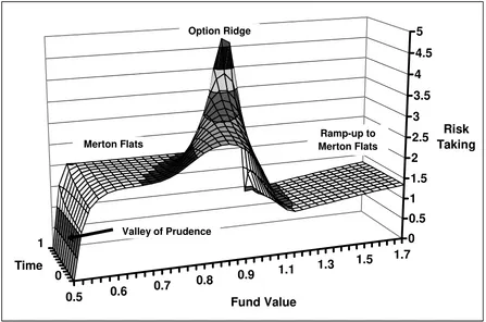
The liquidation boundary effectively turns the manager’s compensation structure into a

knockout call. With our standard parameters, there is a “rebate” equal to equation (2) if the lower

boundary is hit. For those parameter values, we depict the manager’s optimal risk-taking in

Figure 1. The manager clearly wants to avoid hitting the liquidation boundary and dramatically

lowers portfolio risk for the fund as she approaches that lower boundary. We have labeled this

region the “Valley of Prudence,” and one can see that the manager is moving all the way to a

purely riskless investment strategy just above the liquidation boundary.

[Figure 1 about here]

Just above the Valley of Prudence, we have a “Merton Flats” area where the manager

chooses an optimal risky investment proportion of 2. This represents an area where fund value is

far enough from the liquidation boundary (given the time left to her evaluation date) that the

possibility of liquidation plays essentially no role in her decision making. In the absence of an

incentive option, Merton Flats would stretch across the rest of Figure 1. However, an incentive

option introduces new features to the landscape.

There is now a region with high proportions invested in the risky asset, which we term

“Option Ridge”. This region is centered just below the high-water mark of H= 1. The manager

is trying to increase the chance of her incentive option finishing substantially in-the-money. She

thus increases the risky investment proportion considerably if the fund value is either somewhat

below or even slightly above the strike price. This incentive tails off rapidly as the fund value

lock-in style behavior seen above Option Ridge. In what follows, we will use lock-in style

behavior to refer generically to reduced risk-taking in the region above Option Ridge, with the

manager choosing risky investment proportions below the Merton optimum. Her motivation is to

reduce the probability of the option falling out-of-the-money. At still higher fund values, far to

the right, there is also another Merton Flats region. To reach that upper Merton Flats, the

manager’s incentive option has to be sufficiently deep in-the-money that it acts like a fractional

share position.

Some recent papers examine effects of incentive compensation on optimal dynamic

investment strategies for money managers. Carpenter (2000) and Basak, Pavlova, and Shapiro

(2006) focus directly on this issue for mutual funds. Goetzmann, Ingersoll, and Ross (2003)

focus primarily on valuing claims (including management fees) on a hedge fund’s assets. These

three papers all obtain analytic solutions using equivalent martingale frameworks in continuous

time. However, they generate seemingly conflicting results regarding the manager’s optimal

risk-taking behavior. We can shed light on the differing results in the above papers by relating them

to our Figure 1. It turns out that these papers have (sometimes rather subtle) differences in how

they model the manager’s compensation structure. We will now highlight how the compensation

structure is being modeled in each of those papers and how those different choices alter risk

taking.

Carpenter (2000) has a risk averse money manager whose terminal wealth is composed of

a constant amount (external wealth and a fixed wage) plus a fractional call option on the assets

under management with a strike price equal to a specified benchmark. That model can be

reinterpreted in a hedge fund context with the benchmark corresponding to the high-water mark.

Carpenter’s model with her standard call replaced by a binary “asset or nothing” option plus the

addition of an implicit managerial share position in the fund.

Both Basak, Pavlova, and Shapiro (2006) and Carpenter (2000) find extreme risk-taking

near the strike price (our Option Ridge) with a dramatic lowering of risk (lock-in behavior) at

somewhat higher fund values followed by gradually increasing risk-taking at still higher fund

values leading up to what we would call the upper Merton Flats region. In other words, both

these models generate behavior similar to what we see above the high-water mark in Figure 1.

Below the strike price, Basak, Pavlova, and Shapiro (2006) find risk-taking that declines

to a constant Merton-style investment strategy when the fund value is far enough below the strike

price so that the option effectively plays no role in the manager’s decision making. In contrast,

Carpenter (2000) finds risk-taking that increases without limit as fund value declines below the

option strike price toward zero. This difference is due to the manager’s implicit share position in

Basak, Pavlova, and Shapiro (2006), while Carpenter’s manager has neither a share position nor

any other incentive (such as a liquidation boundary) to reduce risk-taking in the lower portion of

the state space. Rather, her manager is motivated only by the probability of getting back into the

money prior to the evaluation date. The further out-of-the-money and the shorter the time to

maturity for her incentive option, the more the manager is willing to gamble.

Neither of these two papers has a lower liquidation boundary. However, such a boundary

is incorporated in Goetzmann, Ingersoll, and Ross (2003). One section of that paper has the state

space of fund value split into regions and the manager is allowed to choose a different volatility

for each region. At their liquidation boundary, fees go to zero. If the objective of the manager is

to maximize fees, such a boundary is to be avoided; and this drives their result that volatility

should be decreased as asset values approach the boundary. This result is similar to our Valley of

Comparison of these models highlights the importance of seemingly minor changes in the

manager’s compensation structure. For example, whether or not the manager has a share position

as well as an incentive option can substantially mitigate risk-taking behavior – compare our

results and those of Basak, Pavlova, and Shapiro (2006) with the more extreme risk-taking in

Carpenter (2000). The nature of the incentive option (e.g. plain vanilla call versus binary

asset-or-nothing) also makes a difference, with the binary option inducing more dramatic shifts in

risk-taking because of the jump in value at the strike price. On the other hand, both types of options

appear to motivate lock-in style behavior slightly above the high-water mark. It is also clear that

liquidation barriers can have major effects. Our Figure 1 may not depict the “whole elephant,”

but it is more general than previous one-period models and illustrates how managerial behavior

can vary dramatically in different parts of the state space.

IV. Endogenous Shutdown

Instead of simply using a prespecified liquidation boundary, we adapt the model to

include a managerial shutdown option. This is an important and realistic extension which

provides a mechanism consistent with a potentially nontrivial number of hedge fund liquidations.

Getmansky, Lo, and Mei (2004) report an 8.8% average annual attrition rate for funds in the

TASS database during 1994-2003. This rate represents funds dropping from the TASS database

for a variety of possible reasons. However, it is clear that a large fraction of the funds were

liquidated. In contrast, the Valley of Prudence and the Goetzmann, Ingersoll, and Ross (2003)

result of reducing risk-taking to zero approaching the lower boundary imply that liquidation at

such an exogenous boundary can be avoided. There are ways to have liquidations with an

deter rapidly reducing risk-taking to zero. However, one would still anticipate a relatively small

number of such forced shutdowns. An endogenously chosen shutdown seems more consistent

with the rather high liquidation rate.

An endogenous shutdown choice represents an American-style option where the manager

can choose to liquidate the fund at asset values above the prespecified lower boundary. Brown,

Goetzmann, and Ibbotson (1999) argue that this might happen because it appears unlikely that

performance will reach the high-water mark (presumably within a “reasonable” time frame). The

problem of covering fixed costs with management fees when fund value is low as well as

marketing difficulties associated with a poor track record can also contribute to the exit decision.

Whether the manager will choose to shut down the fund depends on her other

opportunities relative to continuing to manage the fund. This would include the possibility of

starting a new hedge fund (with a new high-water mark) as well as other alternatives such as

accepting outside employment. On the other hand, keeping the fund alive preserves the

possibility of earning an incentive fee by exceeding the high-water mark. Also, the manager may

desire to invest her own capital using the fund’s superior return technology and may not be able

to do so unless the fund remains in existence. This could be due to scale economies (e.g. an

expensive trading platform) or legal considerations.

We model her outside opportunities in a simple manner, using L to represent an annual

compensation rate which is independent of the fund value. If the manager chooses to shut down

the fund at time τ with a fund value Xτ , she receives at maturity:

The first two terms of (6) indicate that the manager recovers her share of the fund aXτ

plus a prorated fraction of the management fee (with no incentive payment). She also earns L

prorated over the time remaining until T. As we work backward in time through our grid, we

compare the utility of receiving (6) with that from choosing the optimal κ(X,t) and continuing

to manage the fund. When the utility of (6) dominates, it indicates the manager would

voluntarily choose to shut down the fund at that fund value and point in time.

[Figure 2 about here]

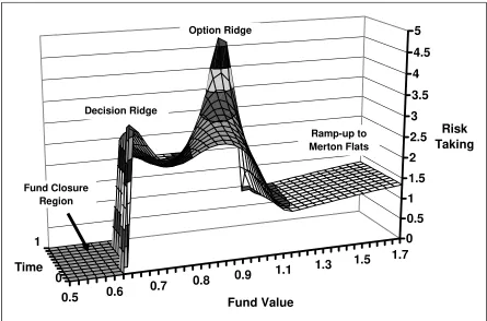
In Figure 2, we illustrate a typical situation with endogenous shutdown occurring at fund

values well below the lower edge of Option Ridge. In that closure region, the probability of

reaching the high-water mark would have been very small. We also see some gambling slightly

above the voluntary closure level along what we have labeled “Decision Ridge.” Here, the

manager is in a situation that could be described as “heads: I win, tails: I don’t lose very much”

due to the partial floor on her compensation provided by outside opportunities. When the value

of her outside opportunities is sufficiently low, the manager will not voluntarily choose to shut

down and must be forced to liquidate the fund at the lower boundary.

Note that if a shutdown occurs, outside investors incur a resetting of their high-water mark

when switching to another fund. In effect, they are forced to forgo the possibility of gains in the

current fund without triggering incentive fees. Moreover, outside investors can experience a

pattern of heavy gambling along Option Ridge with fund closure at perhaps only slightly lower

asset values – leading to a reset of their high-water mark. To assess the likelihood of such a

situation, an outside investor needs to be able to address the manager’s optimal actions in an

V. Managerial Behavior with Multiple Evaluation Periods

Our basic model considers only a single evaluation period, and this may lead to more

dramatic swings in managerial risk-taking than would occur with a sequence of performance

evaluations. This is also true for Carpenter (2000) and Basak, Pavlova, and Shapiro (2006). In a

multiyear framework, the manager would consider not only fund performance to the next

evaluation date but also potential subsequent compensation based on fund performance in later

periods. This should dampen extreme risk-taking. If the fund performs poorly during the

previous year, it reduces expected future compensation since the manager will be starting next

year with that next year’s incentive option out-of-the-money. Also, the convexity (“gamma”) of

a European option is a decreasing function of time to maturity and declines rapidly for

near-the-money options. Furthermore, options which are substantially out-of-the-near-the-money have relatively

low convexity. Hence, options maturing in future years will have current managerial behavior

effects roughly analogous to additional share positions. Again, this will serve to dampen

risk-taking in earlier periods.

Panageas and Westerfield (2005) examine this issue and indeed obtain results that the

manager should optimally have a constant risky investment proportion. However, the continuous

time and continuous state space structure of their model means that each option is of only

infinitesimal size and each evaluation period is instantaneous. So one issue is whether their basic

result holds with annual evaluation periods (as in practice) and options of substantial size.

Another important issue is boundary behavior that alters their result. Their fund can be

shutdown independently of fund value at a random future date determined by an exogenous

realistic way to model that is with an endogenous liquidation decision. The high rate of hedge

fund closures suggests that we should model this aspect of fund management. Consequently, we

use our endogenous shutdown approach as a lower boundary in the following analysis with

multiple yearly evaluation periods.

Building a model with multiple evaluation periods is challenging because there is a path

dependency in the high-water mark. The last evaluation period is simply our standard setting as

in Figure 2 above. In earlier years, the manager’s compensation at year end (management and

incentive fees for that year) needs to be augmented by the certainty equivalent of the indirect

utility of continuation. For year-end fund values below the high-water mark, the indirect utility

of continuation is simply the next year’s indirect utility measured at the initial fund value equal to

the previous year’s ending value. For year-end fund values above the high-water mark, the

situation is a little more complicated since the high-water mark gets reset. We calculate the

certainty equivalent for such a (relatively high) fund value as equal to the continuation certainty

equivalent at the high-water mark times the ratio of new (relatively high) fund value to the high

water mark. We are able to use this relatively simple procedure due to our assumption of power

utility (more details are provided in the Appendix).

[Figure 3 about here]

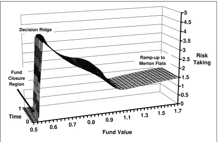
Figure 3 displays the pattern of optimal managerial risk-taking over the next year, starting

3 years from the terminal date of the analysis. If the fund is not shut down, the manager receives

the annual management fee and a potential performance incentive at the end of this evaluation

with the same compensation structure before the final one-year period which is then identical to

what we displayed in Figure 2.

Comparing Figure 3 with Figure 2, we can see that Option Ridge has been pushed

downward and is no longer discernable. This result actually takes two years, and a smaller

Option Ridge would still be visible in a display for the intervening year. Decision Ridge is still a

prominent feature but it has moved downward, with fund closure at lower levels. While there is

considerable variation in risk taking across different fund values in Figure 3, there is now much

less variation as a function of time until the next evaluation date.

If we were to move backward in time, modeling more and more years until the fund’s

terminal date, we would see essentially the same pattern as in Figure 3. This continues until

Decision Ridge bumps against some hard exogenous liquidation boundary. Then Decision Ridge

starts getting pushed downward (over several years) and a Valley of Prudence starts extending

upward from the exogenous liquidation boundary. Eventually, the pattern of managerial behavior

can be described as a Valley of Prudence starting at the exogenous lower boundary and sloping

slowly upward to a Merton Flats area at substantially higher fund values. However, this whole

process can take a very long time. For our standard parameters, it takes over 30 years for

Decision Ridge to bump up against an exogenous liquidation boundary set at 0.25.

VI. Concluding Comments

A useful way of interpreting our results is to consider the perspective of a hedge fund

investor with CRRA utility, who would always prefer a Merton Flats strategy with constant

proportional risk-taking. We find that the industry-standard compensation contract induces

On the other hand, when she has a longer horizon with several annual evaluation periods, her

optimal investment strategy is substantially closer to a constant proportion as long as the fund is

performing reasonably well. The much-debated incentive effects stemming from option-like

compensation thus die out relatively quickly. If fund value has declined to a level where fund

closure is a serious possibility, she begins moving toward much higher risk portfolios along

Decision Ridge. This behavior carries through strongly with horizons of many years, even

decades. Given the high rate of hedge fund closure, this implication of endogenous shutdown

seems particularly important for understanding investment management at hedge funds.

The risk-taking behavior we find is much richer than what can be generated by one-period

models such as Carpenter (2000) and Basak, Pavlova, and Shapiro (2006) or models with

instantaneous valuation periods such as Goetzmann, Ingersoll, and Ross (2003) as well as

Panageas and Westerfield (2005). This results from our ability to solve the American-style

option problem needed to implement endogenous shutdown as well as developing a procedure for

realistically handling multiple discrete evaluation periods with path dependent high-water marks.

We feel this indicates the direction to proceed in analyzing similar incentive issues in the future.

From a policy perspective, it is clear that the typical hedge fund contract plus managerial

control of fund investment positions can result in dramatic risk taking as the manager tries to

increase the probability of her incentive option finishing substantially in-the-money. This

behavior near the high-water mark is much more pronounced when the manager does not own

shares (implicitly or explicitly) in the fund. On the other hand, such behavior is diminished when

the manager anticipates an extended career with the fund and many evaluation periods – hence, a

sequence of incentive options. It is important that fund investors understand this structure.

Typically, managerial risk taking that more closely approximates investor preferences can be

Endogenous shutdown also induces a nonlinearity in the manager’s compensation.

Effectively, the manager has an American put option. Again, it is important for fund investors to

understand this phenomenon. If a fund has been performing poorly, the likelihood increases for

endogenous shutdown preceded by increased risk taking. Controlling such risk taking could be

difficult; however, contractual limits on leverage or verifiable risk management constraints

Appendix: Numerical Procedure

Optimal control of a stochastic process in an investment context is a discrete-time

descendent of Merton (1969). Merton’s work in turn is based on Markowitz’s (1959) dynamic

programming approach and Mossin’s (1968) implementation of that idea in discrete time.

According to Kushner and Dupuis (1992), the models of choice in the stochastic control literature

are Markov chain models where the state variable evolves on a finite grid according to transition

probabilities from a Markov chain. A state of the art implementation is Jarvis and Kushner

(1996) with the drift linear in the control, constant volatility, and controls which are state

dependent but constant over time. Our model is also a Markov chain model, albeit on an open

grid since we have no upper boundary for our fund value state variable. Our problem is,

however, much harder then Jarvis and Kushner (1996) – primarily because our control is both

time and state dependent. We also have a log asset value process with drift and volatility being

nonlinear and linear in the control, respectively.

The basic structure of our model uses a grid of fund values X and time t, with ∆(log X)

constant as well as time steps ∆t of equal length. The initial fund value X0 is on the grid, and

we choose the grid spacing such that ∆(log X) is equal to r∆t. This choice implies that in the

limiting case where κ = 0 (the manager chooses to only invest in the riskless asset) the value

process will still reach a regular grid point.

To calculate expected utilities, we will need the probabilities of moving from one fund

value at time t to all possible fund values that can be reached at t+∆t. The possible log X

moves are i∆(logX). We use i to index the grid points to which we can move. In the current

implementation, the range for i is from –60, …, 0, …, 60. The probabilities for those possible

for X over the next time step. The risky investment technology has a constant growth rate of µ

and a standard deviation of σ. The riskless investment grows at the constant rate r. The

parameters µ, σ and r can be deterministic functions of (X,t) without generating much

additional insight about managerial risk-taking. For a given kappa, the log change in X is

normally distributed with mean 1 2 2

, t [ (1 )r 2 ] t

κ

µ ∆ = κµ+ −κ − κ σ ∆ and volatility σκ,∆t =κσ ∆t.

Note that this mean and variance do not depend on the level of X. They do depend on ∆t but

not on t itself. Since the normal distribution is characterized by its mean and variance, the

probabilites we need are solely functions of κ and not the level of X or time.

We now use the discrete normal distribution. For a given κ, we calculate the

probabilities based on the normal density times a normalization constant so that the computed

probabilities sum to one:

(A1)

2

,

, ,

, , ₂

60

,

60 , ,

(log ) 1 1 2 2 (log ) 1 1 2 2 t t t i t t

j t t

i X EXP p j X EXP κ κ κ κ κ κ κ µ σ πσ µ σ πσ ∆ ∆ ∆ ∆ ∆ =− ∆ ∆ ⎡ _{⎛ ∆ − ⎞} ⎤ ⎢_{− ⎜⎜ ⎟⎟} ⎥ ⎢ _{⎝ ⎠} ⎥ ⎣ ⎦ = ⎡ _{⎛ ∆ − ⎞} ⎤ ⎢_{− ⎜⎜ ⎟⎟} ⎥ ⎢ _{⎝ ⎠} ⎥ ⎣ ⎦

∑

We keep a lookup table of the probabilities for different choices of κ, which we vary

from 0.2 to 5 in steps of 0.01 and where we include 0 in order to allow the risk free

investment strategy. However, the ends of this range could be problematic and result in poor

approximations to the normal distribution. For low κ values, the approximation suffers from not

having fine enough fund value steps. For high κ values, the difficulty arises from potentially not

To insure reasonable accuracy, we compare the standardized moments of our

approximated normal distribution ˆµ_j with the theoretical moments of the standard normal,

1 3 ... ( 1)

j j

µ = ⋅ ⋅ ⋅ − for j even and µ_j =0 for j odd. In particular, we calculate a test statistic

based on the differences of the first 10 approximated and theoretical moments scaled by the

asymptotic variance of the moment estimation (Stuart and Ord (1987), p. 322):

(A2)

2 10

0

2 2 2

1

1 2 2 1 1 1

ˆ 1

, where we set 1 and 0.

10 ( 2 )

j j

j n j j j j j

n

j j

µ µ

µ

µ µ µ µ µ µ

= − − + ⎛ − ⎞ = = ⎜ ⎟ ⎜ _{− + −} ⎟ ⎝ ⎠

∑

After some experimentation, we discard distributions with risky investment proportions of less

than 0.2. We finally have a matrix of probabilities with a probability vector for each κ value in

our remaining choice set.

We now calculate the expected indirect utilities and initialize the indirect utilities at the

terminal date JT to the utility of wealth of our manager UT(WT) where her wealth is solely

determined by her compensation scheme. Our next task is to calculate the indirect utility function

at earlier time steps as an expectation of future indirect utility levels. We commence stepping

backwards in time from the terminal date T in steps of ∆t. At each fund value within a time

step t, we calculate the expected indirect utilities for all κ values using the stored probabilities

and record the highest value as our optimal indirect utility, JX,t. We continue, looping backward

in time through all time steps.

In our situation, using a lookup table for the probabilities associated with the κ’s has two

advantages compared with using an optimization routine to find the optimal κ value. For one,

a global optimization method that will find the true maximum even for non-concave indirect

utility functions. In such situations, a local optimization routine can get stuck at a local

maximum and gradient-based methods might face difficulties due to discontinuous derivatives.

When implementing our backward sweep through the grid, we have to deal with behavior

at the boundaries. The terminal step is trivial in that we calculate the terminal utility from the

terminal wealth. The lower boundary is also quite straightforward. We stop the process upon

reaching or crossing the boundary and calculate the utility of the payment associated with hitting

the boundary at that time U(Wτ). We use these values in calculating the expected indirect utility

at earlier time steps.

For the numerical implementation, we also need an upper boundary to approximate

indirect utilities associated with high fund values. We use a boundary 1200 steps above the

initial X0 level. For fund values near that boundary, our calculation of the expected indirect

utility will try to use indirect utilities associated with fund values above the boundary. We deal

with this by keeping a buffer of fund values above the boundary so that the expected indirect

utility can be calculated by looking up values from such points. We set the terminal buffer values

simply to the utility for the wealth level associated with those fund values. We then step back in

time and use as our indirect utility the utility of the following date times a multiplier which is

based on the optimal Merton (1969) solution without consumption:

2 2

exp[∆t(µ−r) (1−γ) /(2γσ )]. We do not assume that these values are correct, but they work

very well. This approach is potentially suboptimal, which biases the results low. However, the

distortion ripples only some 30 – 70 steps below the upper boundary, affecting mainly the early

time steps.

Finally, we turn our discussion to the implementation of the multiple-year evaluation

year X1 is at or below fund value at the beginning of that year X0, then the high-water mark is

not reset (H1 = H0). The second year’s continuation indirect utility is then simply the indirect

utility J(X1) of starting that second year at X1 and having a one-year horizon remaining. We

convert this J(X1) to a certainty equivalent value U-1[J(X1)] and add it to the compensation for

year one (W1), which in this case is just the management fee. We then calculate the total

indirect utility U W

{

}

Finally, we need to deal with the situation where the high-water mark has been reset.

With power utility, managerial behavior for the following period will be the same as simply

starting that second period at a high water mark of 1. Here we assume that the lower boundary is

also rescaled to the same extent as the high-water mark so that the lower boundary is always half

the high-water mark 0.5H. However, the manager’s shares (plus management and incentive

fees) will be worth more due to the greater fund value. Since we know the indirect utility of

starting with a high-water mark of 1, we simply scale the associated certainty equivalent by the

ratio of the higher fund value and the old high water mark of 1. The above argument can now be

References

Basak, S., A. Pavlova, and A. Shapiro. “Optimal Asset Allocation and Risk Shifting in Money

Management.” Review of Financial Studies, forthcoming (2006).

Brown, S. J., W. N. Goetzmann, and R. G. Ibbotson. “Offshore Hedge Funds: Survival and

Performance, 1989-95.” Journal of Business, 72 (1999), 99-117.

Brown, S. J., W. N. Goetzmann, and J. Park. “Careers and Survival: Competition and Risk in the

Hedge Fund and CTA Industry.” Journal of Finance, 61 (2001), 1869-1886.

Carpenter, J. N. “Does Option Compensation Increase Managerial Risk Appetite?” Journal of

Finance, 55 (2000), 2311-2331.

Fung, W., and D. A. Hsieh. “A Primer on Hedge Funds.” Journal of Empirical Finance, 6 (1999),

309-331.

Getmansky, M., A. W. Lo, and S. X. Mei. “Sifting Through the Wreckage: Lessons from Recent

Hedge-Fund Liquidations.” Journal of Investment Management, 2 (2004), 6-38.

Goetzmann, W. N., J. E. Ingersoll, Jr., and S. A. Ross. “High-Water Marks and Hedge Fund

Hu, P., J. R. Kale, and A. Subramanian. “Fund Flows, Performance, Managerial Career Concerns,

and Risk-Taking: Theory and Evidence.” Working paper, Georgia State University, (2005).

Jarvis, D., and H. Kushner. “Codes for Optimal Stochastic Control.” Documentation and Users

Guide, Brown University, (1996).

Kushner, H., and P. Dupuis. Numerical Methods for Stochastic Control Problems in Continuous

Time. Berlin and New York: Springer Verlag (1992).

Markowitz, H. Portfolio Selection: Efficient Diversification of Investments. Cowles Foundation

Monograph #16: Wiley (1959) (reprinted by Blackwell 1991).

Merton, R.. “Lifetime Portfolio Selection under Uncertainty: The Continuous Time Case.”

Review of Economics and Statistics, 51 (1969), 247-257.

Mossin, J. “Optimal Multiperiod Portfolio Policies.” Journal of Business, 41 (1968), 215-229.

Panageas, S. and M. M. Westerfield. “High-Water Marks: High Risk Appetites? Convex

Compensation, Long Horizons and Portfolio Choice.” Working paper, University of Southern

California, (2005).

Stuart, A., and S. Ord. Kendall’s Advanced Theory of Statistics. Vol. 1, 5th ed., New York:

Table 1. Standard Parameters

Time to maturity T 1 Interest rate r 0.0578

Log value steps below/above X0 600/1200 Initial fund value X0 1.00

Risk aversion coefficient γ 4 Mean µ 0.0778

Number of time steps n 50 Volatility σ 0.05

Initial high-water mark H 1.00 Incentive fee rate c 0.20

Liquidation boundary Φ 0.50 Basic fee rate b 0.02

Manager’s share ownership a 0.10

Future nodes for the Normal approx. 1+2×60 = 121

Figure 1. Optimal Risky Investment Proportion in One-Period Reference Case

In this figure, the manager receives a management fee (b = 2%), an incentive option (c = 20%),

and also has an equity stake (a = 10%). Other parameter values are as specified in Table 1.

0.5 0.6 0.7

0.8 0.9 1.1

1.3 1.5 1.7 0 0.5 1 1.5 2 2.5

3 3.5 4 4.5 5

Risk Taking

Fund Value Option Ridge

Ramp-up to Merton Flats

1 Time

0

Figure 2. One-Period Optimal Risky Investment with Endogenous Shutdown

In this figure, the manager receives the standard compensation package: a management fee (b =

2%), an incentive option (c = 20%), and also an equity stake (a = 10%). She can also choose to

voluntarily shut down the fund to pursue an outside opportunity with an annual compensation of

0.018. Other parameter values are as specified in Table 1.

0.5 0.6 0.7

0.8 0.9 1.1

1.3 1.5 1.7 0 0.5 1 1.5 2 2.5 3 3.5 4

4.5 5

Risk Taking

Fund Value Option Ridge

Ramp-up to Merton Flats

1

Time 0 Fund Closure

Region

Figure 3. Optimal Risky Investment During an Earlier Evaluation Period

This figure displays risk-taking during a one-year evaluation period starting three years before the

final evaluation date. Each year is an evaluation period with the manager having the standard

compensation package: a management fee (b = 2%), an incentive option (c = 20%), and also an

equity stake (a = 10%). She can also choose to voluntarily shut down the fund to pursue an

outside opportunity with an annual compensation of 0.018. Other parameter values are as

specified in Table 1.

0.5 0.6 0.7

0.8 0.9 1.1

1.3 1.5 1.7 0 0.5 1 1.5 2 2.5 3 3.5 4 4.5 5

Risk Taking

Fund Value Fund

Closure Region

Ramp-up to Merton Flats

1 Time

0