The Pollutant Spreading Model AUSTAL 2000
Is Not Validated
Rainer Schenk
Rosenberg 17, D-06198 WETTIN-Löbejün, Germany
Copyright©2017 by authors, all rights reserved. Authors agree that this article remains permanently open access under the terms of the Creative Commons Attribution License 4.0 International License
Abstract With individual examples [1 to 4] Schenk has
demonstrated for AUSTAL2000 that the II. Law of Thermodynamics and the mass conservation law are violated. In [5] Truckenmüller et. 13 alii one contradicts and explains that AUSTAL is verified and validated yet. However, it turns out that there is a trivial solution in the posted derivation of the reference solution. It will be noted that this solution is not usable and performs speculative deposition rates and thus hurts the balancing differential equation. The correct nontrivial solution, which is suitable for the description of deposition and sedimentation are given in this paper. Beyond the generality of the earlier objections raised against AUSTAL occupied by valid integral theorems. They are not restricted to individual cases. Homogeneity tests turn out to be useless trivial cases and are not suitable for validation. For identical tasks, different solutions are given and direct users astray. It is claimed to have taken into account sources at 200m height, but the simulation results do not show the effect of high altitude sources. Criticizable terminology shows that the authors of AUSTAL have little busy with the basics of momentum, heat and mass transfer laws. In the context of other inconsistencies, the author concludes that the grounds given by Janicke & Janicke tests to sedimentation and deposition uniformity and could not have taken place. The life story of AUSTAL 2000 begins in 1984 with a fatal error and via LASAT to AUSTAL. She has found in 2016 a temporary end with an unprecedented sleight of hand. Mathematics and mechanics are used as valid tools of an incorruptible evidence.Keywords Air Pollution, Spread of Air Pollutants,
Emissions, Particle Model, Deposition, Sedimentation, AUSTAL20001. Introduction
To assess and review of the primary literature AUSTAL stands for [7] Janicke L. et al., [8] Janicke, [9] Janicke L., [10] Janicke U. et al., [11] VDI RL [12] Heimann, [13] and R.
Röckle [14] Thielen H. et al. available. Other bases for modeling the propagation of air pollutants and for program developments are et.al. in [15] Axenfeld F. and [16] IB Janicke described. The relevant reports on the development and description of AUSTAL for [8 to 10] have been drawn little manageable. The reader must gather individually, the mathematical and physical foundations of all reports. About development, practical application, claim and prognosis of AUSTAL can be found in [17] L. Janicke. With AUSTAL as their integral part ([18] TA Luft) was set in 2002 in force in the Federal Republic of Germany, the new TA Luft.
achieved at the end of 10 days, the stationary solutions, what is true for a single instance of the specified comparative calculations for deposition and sedimentation and homogeneity?
Between the beginning of the development AUSTAL in 1981 and entry into force of the new Technical Instructions on Air Pollution Control (TA Luft) in 2002, 21 years have passed. According to [17], if you want to meet again, to think about how the TA Luft is to make air in the next 20 years prognostically. Including various developments has been made continuing to the present. A completed and located in the new development application relates AUSTAL in version 2.5, odor dispersion, according to [20] Janicke. To validate this model development identical reference solutions to sedimentation and deposition and homogeneity are indicated, one of which was established already in the described cases that they are not suitable for all erroneous and comparative calculations. Also on the proven faulty stationary simulation times of 10 days and on the BERLJAND profiles allegedly used is referenced. Neither subjected to the trouble to describe the physical peculiarities of the odor propagation, nor will this given appropriate reference solutions. Physically based different model approaches are ignored and little described. Only in [15] a rather adventurous conceptual model is described, for example to describe the deposition what the erroneous reference solutions declares. Further developments relate, for example, an online system for a nuclear power plant remote monitoring system, a software system for simulation and inhalation of radionuclides (LASAIR) and Airport induced to estimate emissions (LASPORT). Whether one uses the same incorrect reference solutions in the case of LASAIR and LASPORT, is not known. In addition, new developments for the calculation of concentration fluctuations by kinematic simulation of atmospheric turbulence and modeling of wet deposition reversibly dissolved gases are available. However, apparently only know the authors of AUSTAL what is to be understood.
In [5] one tries to refute the objections [1 to 4] levied in and refer to various VDI guidelines and regulations. Textbook knowledge is not used. Simultaneously, the derivation of questionable reference solution will be published. In this paper it is demonstrated that this is wrong. The correct solution is given. By means of valid integral theorems is proved that the objections raised in [2] are universal and applicable not only to the described individual examples. In [6] Trukenmüller you deal with the objections raised, however, cannot detect the faulty implementation in [4]. For this reason, you want to at least demonstrate the equivalence, but one is unable to prove equivalence. The diversity is maintained and all contradictions are not invalidated. If the universality is demonstrated, it is not difficult to show further inconsistencies. These relate here all the case studies with "volume source over the entire
computational domain", contradictory solutions in homonymous tasks and faulty solution curves in the case of high altitude sources. Criticizable terminology that the authors of the AUSTAL is required for modeling and calculation of the spread of air mixed in basic knowledge of the theory of momentum, heat and mass transfer inadequately available. In summary, the author comes to the conclusion that verification of AUSTAL could not have taken place.
The following considerations are based on the test case 11 for uniformity, the case 22a, sedimentation without deposition, and to the case 22b, with deposition sedimentation. All case studies refer to illustrations and descriptions for [8+ to 10]. As part of a root cause analysis the incorrect model assumptions of the authors of AUSTAL are described.
2. Trivial Reference Solution after
Janicke & Janicke
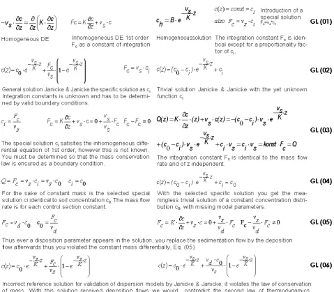
The authors of AUSTAL consider a one-dimensional stationary propagation process for validation. This is described by the differential equation (01) of Figure 1 and taken into account with the sedimentation rate
v
s a convective and with use of am
i=
−
K
⋅
∂
c
/
∂
x
i conductive transport. It is an ordinary differential equation of second order, for their solution two boundary conditions are required. These are described by a constant concentration in the lowest layerc
0 and by the coincidence of conductivematerial and deposition power on the lower limit. Specification of a constant vertical material flow, which is mistakenly referred to by the authors of AUSTAL as area source, are obtained with the analytical solution, the concentration distribution, the concentration in the lowest layer and the associated sedimentation and deposition flows.
0 d 0
und
v
c
c
v
s⋅
⋅
These analytical relationships are disregarded in the present case, as evidenced below.Figure 1. Incorrect reference solution according Janicke & Janicke
3. Nontrivial Reference Solution by
Schenk
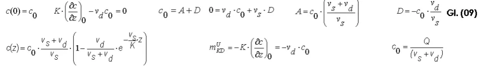
For the in section 2 explained the task, the formula sets the correct derivations of the reference solution are described in figure 2.
The equations (07) are identical to the relations (01), and the solution method with the two integration constants A and D will be commented on by the equations (08). The determination of the constants of integration and derivation
of the relevant non-trivial solution describe the relationships (09). With this solution, the concentrations in the lowest layer and deposition sedimentation streams and the distribution of air admixture can be calculated consistent when specifying a constant mass flow rate,
)
(
0
v
sv
dc
Figure 2. Non-trivial reference solution by Schenk
4. Application of Integral Theorems and
Generality
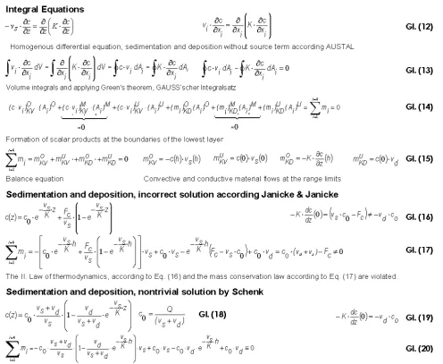
An individual examples was demonstrated for the case studies and sedimentation deposition that the II. main law and the mass conservation law are not met in [2].Means true integral equations can be proved that the formulated objections are universal. In Figure 3, all relevant formula sets are explained. The equations (12) are in turn identical to the original differential equation (01). After formation of
Figure 3. Application of integral theorems on the incorrect solution after Janicke & Janicke and nontrivial solution by Schenk
5. Comparative Calculations
Homogeneity and Sedimentation and
Deposition with "Volume Source over
the Entire Computational Domain"
Are Useless Trivial Cases with Just
Such Solutions
The following considerations of Figure 4 apply to all test cases to homogeneity and on the case example 22a, sedimentation without deposition, in the case of homogeneity here by way of example, the case is considered 11. All these cases have in common that it is considered in the test calculations of the authors of AUSTAL from a "source volume over the entire computational domain". In all other cases, you look curiously enough, notwithstanding, sources, which should have been situated at 200m height.
volume source over the entire computational domain have spatial concentration gradients disappear after equation (22). After that prepare their financial statements the equations (21) and (22) because of the reduced product formation between lack of gradient and a factor somehow a common trivial differential equation with a similar solution, Eq. (24).
The original intention to investigate the influence of homogeneous and inhomogeneous turbulence with these tasks, fails because all solutions of arbitrarily chosen diffusion approaches are independent. For the case study 22a the same observation is true, since the sedimentation rate as
in the previous case, the diffusion equation can have no influence on the solution of the propagation process because of the vanishing concentration here. Not only just so is well founded, that a validation of AUSTAL could not have taken place. All model parameters are, inter alia, described in [8],
which the source term to 0,139μg/(m³ * s) can be calculated
from Eq. (23). That should be so directed consciously astray because of the words "Source volume over the entire computational domain" and erroneous reference solutions of reading, is not alleged.
6. For One and the Same Task Are Two
Different Solutions Indicated
In Section 5 has been shown that reducing the tasks of the cases 11 and 22 on one and the same differential equation (24). After that is independent of all diffusion approaches and sedimentation after3600s the concentration of 500μg/m³
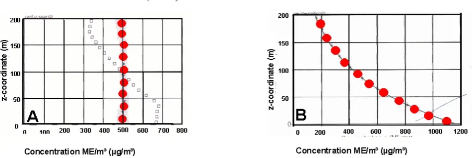
achieved and not after10 days, as indicated by the authors of AUSTAL. At least, after the A graphic Figure 5 and according to [8], p 52, and [9], p 28, the steady state concentration of 500μg/m³ specified correctly. In case 22a
with the same resolution of the case 11 on the other hand, after graphics B after [8], p 56, and [9], p.33, Figure 7, one of the case of 11 different faulty exponential indicated.
It is now before the event that one specifies for one and the same tasks, two different solutions, which must irritate the reader. How so dispersion models to be validated, cannot be explained.
Further studies by [21] Schenk lead to the conclusion that the concentration distribution by graphic B is already defective, and the concentration in the lowest layer has been determined with 1100, 6μg/m³ speculative. Furthermore, the
[image:7.595.66.542.364.524.2]presence of air mixed in is basically to question, since the case 22a by [8], p.56, with the premise of no air admixtures are emitted,
F
c=
0
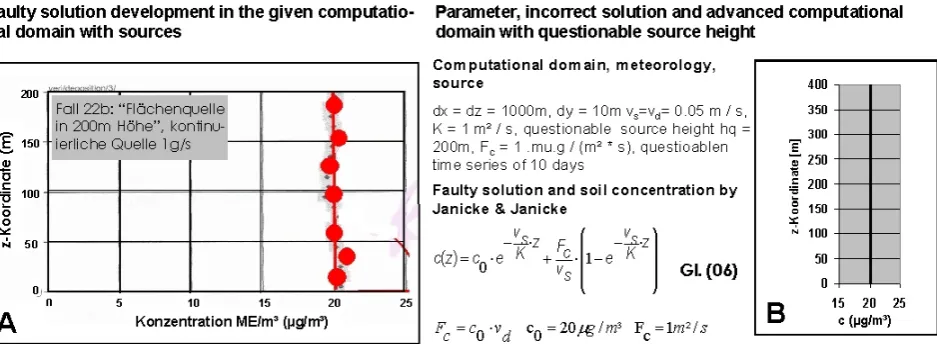
. Also this example shows that a validation of AUSTAL so could not have taken place.Figure 6. Sources are allegedly located in 200 m
7. Supposedly Sources Have Lain at
200m
Unlike the case of example 22a, was in which, as with all homogeneity tests of an assumed "volume source over the entire computational domain", taking into account for [8 to 9] for example calculations 21 and 22b by derogation and unfounded area sources at 200m, but let the purpose
calculated concentration distributions do not recognize the effects of high altitude sources.
Also there is no way to determine the source heights in this specified analytical solutions or vary such as can be seen in the incorrect solution (06) for the reference case 22b. Between the formulated tasks and the reported results are contradictions cannot be overlooked.
opportunity to recalculate the amounts reported by the authors of AUSTAL simulation results considering varied source heights numerically. Comparatively, these results are described in figure 6. The graph A shows the concentration distribution for the case 22b of the authors of the AUSTAL. The upper limit of the control room is limited vertically with 200m. The graph describes the specified propagation parameters and the erroneous reference solution (06) a
constant concentration of 20µg/m³ distribution, which at the
upper boundary at 200m a source should have been lying. In the graph B a similar constant concentration distribution is shown by equation (06), however, the control room has been extended up to 400m in order to represent the effect of possible sources. The presence of a source at 200m is not apparent. Using identical model parameters the bill was repeated, taking into account varied source heights by means of a numerical method. The result shows the graph C where the studied source heights are 100m, 200m and 300m amount. At constant deposition velocity
v
d against the sedimentation ratesv
s are different in the specified interval. The soil concentration for the Reference Case 200m not is20µg/m³ but only 10µg/m³, which can be recalculated with
the correct reference solution (09) and for a constant mass flow rate of the
Q
=
c
0⋅
(
v
s+
v
d)
=
1
m
g
/(
m
²
*
s
)
rd. The error thus amounts to 100%. The influence of different source heights on the concentration distribution is unlike AUSTAL clearly. In addition, it is observed that in the case of a vanishing deposition rate forv
d=
0
m
/
s
of the deposition current disappears. The concentration gradient and hence the conductive material stream at the bottom are also equal to zero, which is in agreement with equation (19). The II. main law and the mass conservation law are met. By contrast, A is the case AUSTAL despite a vanishing concentration by graphics asserts a deposition power can occur. They disregarded that after the II. Law of conductive material flow must coincide with the deposition stream at the bottom. In addition, it can be recalculated, that the mass conservation law is violated. The graph D shows again 200m conditions for the reference case. During indicated by the authors of AUSTAL outlandish for all tests for deposition and sedimentation and homogeneity that all equalization times should have amounted to 10 days is this only 2.6H in the present case. In Figure 6 the complete information on computational domain and meteorology as well as the determined sedimentation and deposition currents are givenfor the reference case. The validity of the mass balance is evidenced by a recalculation.
In conclusion, there is the result that the purpose of the authors of AUSTAL assertion, one would have considered sources at 200m, is not true. The base concentration is calculated incorrectly. It specifies a deposition power would take place, though this cannot occur because of the vanishing concentration gradient at the bottom. The recovery time is calculated incorrectly. Also this information is not true, as can be recalculated. How would like to develop with such eccentricities dispersion models, cannot be explained. The authors of AUSTAL develop this strange model concept. Comparative calculations with a source altitude of 200m have been held.
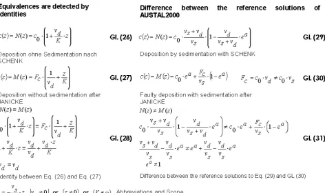
8. Difference between the Reference
Solutions
The inequalities (05), (16) and (17) show that the reference solutions of AUSTAL violate the II. law of thermodynamics and the conservation of mass. In the essay [6], the authors of AUSTAL grapple with this formula set of figures 1, 2 and 3 and cannot identify any error in the derivations. For this reason, we want to demonstrate an equivalence, bringing all inconsistencies have cleared up at least. However it is evident that this is a fallacious argument. Regardless of the statements by [6] to the equivalence of reference solutions should first be pointed out that from the equivalence cannot be spoken. The required matching sets of formulas and the physical principles are described in the figure. 7 The Eq. (29) explains the correct reference solution N (z), while Eq. (30) the faulty AUSTAL solution M (z) explained. To demonstrate equivalence, both solutions are equivalent to the relations (31). With the following result
1
)
exp(
a
≠
is shown that in contrast to the embodiments according to [6] not equivalent and therefore no identity exists. Only in the case of assumptions, which preclude the formulated tasks and physically are preserved, such as a vanishing sedimentationv
s=
0
, an unrealistic diffusionFigure 7. An equivalence between the reference solutions for sedimentation and deposition can not be detected
The valid sedimentation
F
c=
c
0⋅
v
s is alsoinadmissible replaced by the deposition
c
0⋅
v
d so that thedeposition rate
v
d so found as free model parameters is atleast considered in the reference solution. To demonstrate how equivalences can be demonstrated, the equations (26) and (27) are also equated in another case. The analytical relationship according to equation (28) occupies the existing equivalence here. The difference with respect to the derivation according to the equations (31) is evident.
It will enlighten be of interest, as opposed to the relations (31) the apparent equivalence is declared between the reference solutions in [6]. These considerations are of considerable importance in so far as the physically correct description of the deposition has a significant impact on the reliability of all dispersion modeling in general.
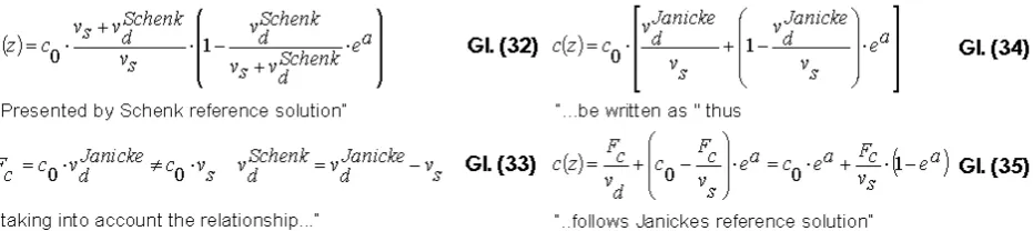
The relevant form sets Eq. (32) to Eq. (35) used in [6] for the proof of equivalence are shown in Fig 8. With the relation (33)
v
dSchenk=
v
dJanicke−
v
s, one would like to prove a supposed equivalence, but the physical validity of this relation is not substantiated. It is also not clear why twodeposition rates must be differentiated,
s Janicke d Schenk
d
v
v
v
=
−
andv
dJanicke.It will enlighten be of interest, as opposed to the relations (31) the apparent equivalence is declared between the reference solutions in [6]. These considerations are of considerable importance in so far as the physically correct description of the deposition has a significant impact on the reliability of all dispersion modeling in general.
Figure 8. difference between the reference solutions
It is still to be clarified, according to which method the relation (33) by [6] is determined. This will also emphasize why a distinction is made between two arbitrary deposition rates. One tries thus bringing about the apparent equivalence, by equating the correct reference solution
N
(
z
)
according to Eq. (37) with the incorrect solution to (36)M
(
z
,
v
d)
and at the same time x replaces the independent parametersd
v
by a dependent parameter x,M
(
z
)
=
N
(
z
,
x
)
. This is it determined as following by a supposed equality.Thus, the relation (33) is calculated as traced by the example of the equations (38). From the equations (38)
follows the equation (33)
v
dSchenk=
v
dJanicke−
v
s if one finally renaming again the variables,x
=
v
dSchenk andJanicke d d
v
v
=
. By one would solve the conflicting task conversely get the equivalent relationship. It turns out that an equivalence is merely tricked in this way,)
(
)
,
(
z
x
N
z
apparent equivalence is well thought out and well planned, but it serves no purpose. In conclusion, one can regard it as proven that there is no equivalence between the reference solutions. it should be to recognize a similarity between the calculated concentration profiles, too, what is not the case.
9. Root Cause Analysis
It can be regarded as undisputed that the derivations of reference solutions for AUSTAL are faulty.
Picture 9. Cause Analysis
Your application for the description of sedimentation and deposition leads to a number of inconsistencies, which have been described by means of suitable formula sets example in Figures 1 to 8. FIG. The evidence is incorruptible. It must be informed of interest with which the erroneous derivation of the reference solution and the futility of all described tests for homogeneity and other comparative calculations of the authors of AUSTAL be explained. In this context it is not irrelevant to determine that was already being used in [15] in 1984 in the "development of a model for calculating the dust precipitation" with an incorrect boundary condition according image 9. One understands there the deposition rate as the "speed with which an upstanding on the ground column containing the deposition capable material by deposition idles." This unconventional idea on the physics of deposition is obviously recognized as a new school of thought and in [25], VDI 1988 "urban climate and air pollution control, a scientific guide for practice in environmental planning" adopted as universally valid. However, the authors of AUSTAL denied that their own definition contradicts all foundations of the theory of momentum, heat and mass transfer. The correct boundary condition for knowing as repeatedly stated in [19] only for completeness. One can no longer trace back when, this formulation was used in process engineering for the first time and included in the teaching. It is the same with the description of the sinking or sedimentation. Thus, for example, according to equation (01) this provided for the entire scope of all balances as a constant, but you do not know that this must be zero because of the no-slip condition
at the lower boundary of the scope of all balances. Due to lack of conceptual model has great difficulty to interpret the results without error here. All other conceptions of authors, for example homogeneity and 3D wind fields are equally absurd to judge. The list of inconsistencies can be continued as desired. That developed in [15] faulty dispersion model has been further developed later to the particle model LASAT, [15] IB Janicke, and later to AUSTAL. This fatal mistake to Figure 9, the life story of AUSTAL2000 begins.
10. Able Criticism Terminology
Subject to the investigations were alone analytical and numerical considerations for solving ordinary differential equations. There is a seminar task instance from the course "Fundamentals of momentum, heat and mass transfer" an academic engineering education with medium difficulty. By analytical solutions are functions continuously described precisely, program developers must prove that their algorithms emulate the analytical solution at a fixed margin of error. However, this presupposes stability, what is nothing to learn in AUSTAL. Instead, we read that solutions may not converge. Criticism of the BERLJAND profile is established, which can be tracked with a study of original literature for [19]. One can learn how deposition processes are physically and mathematically described there. The criticism of the homogeneity test should be faulty. Homogenizing belongs as well as the crushing of the basic operations of process engineering. When homogenizing and crushing the material compensation is effected by an energy input, while in the case of diffusion potential gradient is responsible. When homogenizing you noticed strange vibrations continue at the range limits, which are not further explained. Why the lateral edges must is made periodically? One reason there is this also not. Also edge effects to cause a deviation from the homogeneous turbulence. How this should be done, is questionable. It describes one in [8] S. 53 that bills homogeneous turbulence and spatially variable increment cannot be performed. "The program always chooses homogeneous turbulence a constant time step". Another time, are still carried out according to [9], p.28, Figure 2, invoices in just such homogeneous turbulence and spatially variable increment. House walls are perpendicular to the road and not somehow. Thus, the Euler coordinates are for example particularly suitable for the implementation of flow and dispersion calculations in built-up areas. Unlike AUSTAL "see" dust particles Euler coordinate house walls and do not want to pass. With mass/time, mass/(time*Länge²),
mass/(time*Länge³) and "volume source over the entire
has been described. The transport distances rarely amounts generally below 100km, but more often it. Finally is the dispersion of pollutants along trajectories across continents away also described in [24] Graedel /Crutzen. While qualified prognostic propagation models are the subject of dissertations with scientific advice generally, it has broken in the case AUSTAL another way. According to [10] in 2000 and 2001, the "evaluation system for plant-related immission" presented before a large number of experts invited to three workshops. As you can read there, the workshop had to follow one another closely. "Therefore, there is no time for research." However, contracting and auditoriums need to be able to rely on expertise and scientific thoroughness and Redlich and truthfulness.
11. Conclusions
For all case studies to sedimentation and deposition as well as for all homogeneity tests all computing and model parameters are published in full by the authors of AUSTAL. After all practices of scientific work is directed so that the readers are prompted to confirm the results and conclusions through its own considerations and recalculations announced.
This circumstance is not to be understood that one should trust without it because of the high priority of the project and the principal authority. The authors of AUSTAL have a right to know whether you could confirm the correctness of their ideas or not. In the described cases, validate the confirmation of the proof in [2] remains to be faulty. This assertion turns into its opposite. Misunderstandings do not exist. Right and wrong do not allow misunderstandings. Basic knowledge of the theory of momentum, heat and mass transfer is little used. The objections to AUSTAL have hardens. The verification could not have taken place. Even the authors of AUSTAL could not to have been able. The call made in [2] that safety-relevant statements, which have been determined with AUSTAL, have to be checked was not invalidated by [5]. This finding also applies to all other propagation models, which have been validated with the presently described erroneous reference solution to sedimentation and deposition, as well as with the indicated homogeneity tests or use its computing cores. The life story of AUSTAL 2000 begins in 1984 with a fatal error and via LASAT to AUSTAL. She has found in 2016 a temporary end with an unprecedented sleight of hand.
REFERENCES
[1] Schenk R.: AUSTAL2000-Methode ist fragwürdig validiert, Stein & Kies, Ausgabe 132/September-Oktober 2014, S. 8 bis 9
[2] Schenk R.: AUSTAL2000 ist nicht validiert, Immissionssch utz 01.15, S. 10 bis 21
[3] Schenk R., Markert, B., Fränzle, St.: The Pollutant Spreading Model AUSTAL2000 IS NOT VALIDATED, 7th International Workshop on Biomonitoring of Atmospheric Pollution (BIOMAP7), June 14-19 2015, Lisbon, Portugal [4] Schenk R.: Replik auf den Beitrag „Erwiderung der Kritik
von Schenk anAUSTAL2000 in Immissionsschutz 01/2025“, Immissionsschutz 04.15, S. 189 bis 191
[5] Trukenmüller A. et 13 alii: Erwiderung der Kritik von Schenk anAUSTAL2000 in Immissionsschutz 01/2015, Immissionsschutz 03/2015, S. 114 bis 126
[6] Trukenmüller, A.: Äquivalenz der Referenzlösungen von Schenk und Janicke, Abhandlung Umweltbundesamt Dessau-Roßlau, 2016-03-04
[7] Janicke L.; Klug W.; Rafailides S.; Schatzmann M.; Strimaidis D.;Yamartino R.: Validierung des „Kinematic Simulation Particle Model (KSP-Modell“ für Anwendungen im Vollzug des BImSchG, Bericht 98-295 433 54 des Bundesministerium für Umwelt, Naturschutz undReaktorsic herheit, Hamburg 2000
[8] Janicke: AUSTAL 2000, Programmbeschreibung, Dunum, 2002
[9] Janicke L.: IBJparticle, Eine Implementierung des Ausbreitungsmodells, Bericht IBB Janicke
[10] Janicke U., Janicke L.: Entwicklung eines Modellgestützten Beurteilungssystems für den Anlagenbezogenen Immissions schutz, IBJanicke, 2002
[11] VDI: Umweltmeteorologie, Atmosphärische Dispersionsmo delle. Partikelmodell, VDI 3945, Blatt 3
[12] Heimann D.: Ausbreitung von Spurenstoffenbei
Schwachwindlagen, DLR Oberpfaffenhofen, 2001 [13] Röckle R.: Gebäudeumströmung. IMA Freiburg, 2001 [14] Thielen H.; Martens R.: Beiträge der GRS im Rahmen der
AUSTAL Workshops, Auftr. Nr. 400003 (AG 1983). [15] Axenfeld F., Janicke, L., Münch J.: Entwicklung eines
Modells zur Berechnung des Staubniederschlages, Umweltforschungsplan des Bundesministers des Innern Luftreinhaltung, Forschungsbericht 104 02 562, Dornier System GmbH Friedrichshafen, Im Auftrag des Umweltbundesamtes, 1984
[16] IB Janicke: Ausbreitungsmodell LASAT, Referenzbuch zu Version 2.10, Dezember 2001
[17] Web, Janicke U: AUSTAL2000,http://www.austal2000.de/d e/history.html, http://www.janicke.de/de/products.html [18] TA Luft: Erste Allgemeine Verwaltungsvorschrift zum
Bundesimmissionsschutzgesetz, GMBI, 2002
[19] Berljand M. E.: Moderne Probleme der atmosphärischen Diffusion undVerschmutzung der Atmosphäre, Akademie-Verlag Berlin, 1982
[20] IB Janicke: AUSTAL2000 Geruchsausbreitung im Auftrag von derLandesanstalt für Umweltschutz Karlsruhe, des Niedersächsischen Landesamtes für Ökologie Hildesheim und des Landesamtes NRW Essen, 2011
[21] Schenk R.: AUSTAL2000 ist nicht validiert, neue Entwicklungen bei der Messung und Beurteilung der Luftqualität, VDI Berichte 2250; S. 237 bis242
[22] Eliassen A., Hov O., Isaksen Ivar S. A., Saltbones J., Stordal, F.: A. Lagrangian Long-Range Transport Model with Atmospheric Boundary Layer Chemistry, Journal of Applied Meteorology,Vol. 21 No. 11, Nov. 1982
[23] Eliassen A., Jensen O., Saltbones J.: Das Trajektorienmodell des NILU Institutes und ausgewählte Modellvergleiche, Norwegian Institute for Air Research, Lillestrom, Oktober 1976
[24] Graedel T. E.; Crutzen P. J.: Chemie der Atmosphäre, Spektrum Verlag, Heidelberg, Berlin Oxford, 1994