Special Spline Approximation in CAD Systems of Linear Structure Routing

Special Spline Approximation in CAD Systems of Linear

Structure Routing

i

D. A. Karpov, V. I. Struchenkov*

Department of General Informatics, the Institute of Cybernetics of the Russian Technological University (MIREA), Russia

Received June 29, 2019; Revised September 27, 2019; Accepted October 9, 2019

Copyright©2019 by authors, all rights reserved. Authors agree that this article remains permanently open access under the terms of the Creative Commons Attribution License 4.0 International License

Abstract

approximation of plane curves defined by a sequence of points by a spline of a given type. This task arises when developing methods for computer-aided design of linear structures: railways and roads, trenches for laying pipelines, canals, etc. Its fundamental differences from the problems are considered in the theory of splines and its applications are as follows: spline elements are of various types (straight line segments and circles joined by clothoids), the boundaries of the elements and even their number is unknown; also there are restrictions - inequalities on the parameters of the elements. Continuity of the curve, the tangent, and the curvature is provided. Clothoids are missing if curvature continuity is not required, for example, when designing pipelines. The above mentioned features of the task do not allow using the achievements of the theory of splines and nonlinear programming. We cannot recognize the individual elements of the desired spline by a given sequence of points. Therefore, it is not possible to implement their selection separately. We must search for the spline as a whole. The article presents a mathematical model and a new algorithm for solving the problem using dynamic programming.

Keywords

1. Introduction

The route of a linear structure is a 3D curve, which is traditionally represented by two flat curves: a plan and a longitudinal profile. The projection of the route on the horizontal plane XOY is called its plan, and the longitudinal profile of the route is a graph of the dependence of the coordinate Z on the curve length in plans,

calculated from the starting point to the current one. We will consider the spline with clothoids since the task without clothoids permits considerable simplifications as a special case. Since the Cartesian coordinates of points of a clothoid are expressed by power series, the search for even one clothoid approximating a sequence of points is not an easy task [1]. In widely used CAD, [2-5], design solutions for the plan and profile of the route are set by the designer and can be corrected interactively. An alternative approach is to develop mathematical models, optimization algorithms, and computer programs [6, 7].

Besides, a complicating circumstance is that the required spline does not have to be a single-valued function, unlike the considered splines whose elements are polynomials [8]. Previously, using nonlinear programming, we solved the problem of optimizing the parameters of a spline with clothoids, which was set as the initial approximation [1].

This task is multi-extremal, and its successful solution depends on the quality of the initial approximation. In fact, this is an optimization of the solution given by the designer in some way or another.

The purpose of this article is to present a model and a new spline search algorithm with clothoids, which gives a final solution to simple cases and provides an initial approximation for the application of a nonlinear programming algorithm in difficult cases

2. Task Formalization

A sequence of points on the plane is given. The required approximating curve is a sequence of elements: a straight line, clothoid, circle, clothoid, straight line, etc. (Fig. 1). In such a way, the plan of the route of railways and highways is designed.

Figure 1. The elements of the route plan The curvature of the clothoid as a function of length

varies linearly from 0 to 1 / R, where R is the radius of the circle. Therefore, at the points of conjugation, the elements have not only a common tangent, but also equal curvature. Consistently connecting the given points with straight lines, we build the initial broken line, which is called a “chain” (Fig. 1). The starting and ending points of the spline, as well as the starting and ending directions are considered to be given.

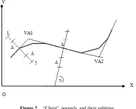
At the vertices of the "chain", we construct normals, i.e. straight lines from the top to the center of the circle connecting three adjacent points (Fig. 2). We remember the angles γi of the normals with the axis OX. To obtain a discrete problem and the subsequent application of dynamic programming on each normal, from the vertex to both sides, we measure an equal number of discrete Δ and then calculate the coordinates of the obtained points.

It is required to find a spline of the specified type, for which the sum of squares of distances hi from the given points of the “chain” to the intersection points of the normals with spline is minimal, that is, min ∑𝑛𝑛 ℎ_𝑖𝑖2 _.

𝑖𝑖=1 Here

n is the number of normals.

Figure 2. “Chain”, normals, and their splitting The following restrictions must be applied: 1. To the radius of the circle R: Rmin≤R≤Rmax.

2. To the length of clothoids Scl: Sclmin≤Scl≤Sclmax and circle Scirmin≤Scir≤Scirmax.

3. To the length of the tangential path Sd: Sdmin≤Sd. Additionally, the following may be set:

 The minimum angle of rotation.

 The range of curvature change rate of each clothoid.  The curvature of the clothoid σ depends linearly on

the length s, measured from the point with zero curvature.

 σ = ks.

 The value of k must correspond to the condition kmin ≤ | k | ≤ kmax. With σ <0 (rotation of the clothoid clockwise) k <0.

Thus, the mathematical model of the problem is as follows:

The objective function is the sum of the squares of the deviations hi of given points from the desired spline It is necessary to find minimum of the objective function with restrictions on the parameters of the spline elements. Any deviation can be calculated when the spline is built, but we do not have a formula for such calculations. Therefore, we have to solve auxiliary problems (for example, the intersection of a straight line and clothoids, see below).

Moreover, the number of spline elements is unknown; therefore, it is impossible to consider the problem of minimizing the objective function as a problem of nonlinear programming. However, there is the possibility of sequentially constructing many options for positioning the vertices of the first rotation angle with inscribed curves, then the first two vertices, then three, etc. In order to avoid a complete enumeration of options, we will use dynamic programming.

The key in dynamic programming concept of “system state” can be defined as following: the starting point of the next left clothoid (in Fig. 1, they are clothoids AB and EF) plus the direction of the side of the angle to which this point belongs. We will search for the starting points of the left clothoid among the numbered points of the normals after splitting them with a given step Δ.

range of angles with discrete ϕ. To this end, in both directions from the angle of the tangent γi + π / 2 we set aside an equal number of discretes ϕ. Thus, a set of directions is formed at each numbered point of each normal. As a result, a set of the "system states" for the application of dynamic programming are formed.

We will need two more quantities: Smin and Smax. This is the minimum and maximum total length of the curve from one “system state” up to another. In Fig. 1, the length of the curve is AB + BC + CD + DE.

Smin = 2Sclmin + Scirmin + Sdmin.

The value of Smax, as well as the discretes Δ, φ and their numbers, while splitting the normals and forming the system states, will be considered as input parameters in order to determine them experimentally with accumulation of operating experience.

By virtue of the features of the task noted above, we do not have an analytical expression of the objective function of any parameters that determine the desired spline. However, for each spline of the desired type, we can check the fulfillment of all constraints and, if they are satisfied, we can calculate all the distances hi, and then the value of the objective function.

3. Frequently Solved Auxiliary

Problems

It is important to emphasize that the restriction on the length of the tangential path creates a relationship between neighboring curves (Fig. 1), which does not allow even with a known position of the VA (hereinafter vertexes of angles) to solve the problem of finding the radius and length of the clothoid for each angle separately. However, this relationship disappears if the beginning of the left clothoid for the next angle is known (point E of Fig.1). In this case, within each angle, we can try to choose the radius of the circle and the length of the clothoid, providing the necessary length of the tangential path. It is the well-known task of “inscribing a curve in a corner”. Therefore, we will strive to reduce the initial variation problem of searching for a spline to the determination of the coordinates of all VA for given starting points of the left clothoids.

In practice, the task “inscribing a curve in a corner” is solved for a given radius. We need to find the radius of the circle and the length of the clothoid. Let us consider how to determine the radius of the curve R and the length of the clothoid s (Fig. 1), observing all the restrictions and minimizing the sum of the squares of deviations from the vertices of the “chain” along the previously constructed normals.

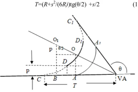
The beginning of the left clothoid (point C in Fig. 3) is known. When a clothoid is arranged, the center of the circle inscribed in an angle is shifted along the bisector on OO1= p / cos (θ / 2). Here p is the distance from the point of tangency of the circle and clothoid to the side of the angle.

With sufficient accuracy for practice, p = s2 _{/ (6R) and} BC = s / 2. For this reason, the distance T from VA with the angle of rotation θ is given by the formula (1):

T=(R+s2_{/(6R))tg(θ/2) +s/2 (1)}

Figure 3. Elements of the inscribed curve.

AA1 and DD1 the arc of the circle before and after fitting of clothoids CD and C1D1, OA is the radius.

The distance from VA to the beginning of the left clothoid on the other side of the corner (point E in Fig. 1) is also known due to the accepted formalization of the concept “system state”, which makes it possible to check the restriction on the minimum length of the tangential path (A1 C1), even before calculating the deviations from the "chain".

We have one equation (1) with two unknowns to determine R and s.

In order to have a solution for the equation (1) with respect to R, it is necessary:

𝑠𝑠<𝑇𝑇/(0.5 +𝑡𝑡𝑡𝑡 �𝜃𝜃

2� √6/3)

Accordingly, we have the following formula for R:

𝑅𝑅=3(2𝑇𝑇−𝑠𝑠)+�9(2𝑇𝑇−𝑠𝑠)2−24(𝑠𝑠𝑠𝑠𝑠𝑠( 𝜃𝜃 2))2

12𝑠𝑠𝑠𝑠(𝜃𝜃₂) (2)

The second root of equation (1) is p = s2 _{/ (6R) and an} outsider.

The length of clothoids in practice is taken as a multiple of 10m.

Since it is not known whether the objective function has local minima, we will iterate over the values of s with a step of 10 m starting from the smallest, calculate R by the formula (2), and check all restrictions including the limit on the radius, on the clothoid parameter k, and on the minimum length of the circular arc. When a clothoid of length s is arranged, the circle inscribed in the angle is shifted along the bisector, and the length of its arc decreases by s.

Therefore, the inequality Rθ-s ≥ Scirmin must be implemented.

on the next side of the angle (in Fig. 1 from point A to point E). We remember the sum, increase s by 10m and repeat the calculation.

It may turn out that a further increase in s does not make sense. In this case, or after exhaustion of the search, we remember s and R, which correspond to the minimum sum. The calculation of deviations requires finding the intersection of the normals with the clothoid, the circle and the straight line. In the latter two cases, the issue has a simple solution. And to search for the intersection of the normal and the arc of the clothoid, we have to organize an iterative process. For example we replace the clothoid with two chords, calculate the intersection of the normal with each of them and leave only one chord for further actions that intersects with the normal, divide it in half, etc. until the length of the search interval is less than the required accuracy. At the same time, to calculate the Cartesian coordinates of the clothoid points, it is necessary to use power series and to recalculate the coordinates from one system to another.

In the Cartesian coordinate system with the center at the point of zero curvature of the clothoid and with the X axis, which coincides with the side of the rotation angle and is directed towards the length increasing of the clothoid, the coordinates of the clothoid points, as a function of the clothoid length, are expressed by rapidly converging power series:

𝑥𝑥=𝑠𝑠(1−𝑠𝑠₄₀4𝑘𝑘2 ₊ 𝑠𝑠8

3456𝑘𝑘4− ⋯

)

𝑦𝑦=s3₆𝑘𝑘 (1- ₅₆𝑠𝑠4𝑘𝑘2 ₊ 𝑠𝑠8

7040𝑘𝑘4− ⋯)

In general, individual subprograms perform the following tasks calculation of:

 the coordinates of the points of two straight line segments intersection;

 VA coordinates and angle of rotation θ;  the circle radius and checking restrictions;

 the coordinates of the point of the normal and the circle intersection;

 the coordinates of the point of the normal and clothoid intersection;

 squares of distances sum from the original points to the spline at the normals.

4. Search Algorithm of the Optimal

Spline

Let us consider a new dynamic programming algorithm for solving the problem of automatic search for VA and inscribed curves.

The concept of "system state" is defined above. At every step of the search, the system may be in different states. The sequence of states, which were selected at each step, forms a trajectory (path). The concept of “state of the

system” is defined by us in such a way that different paths that lead to the same state are comparable, since the sets of their possible continuations coincide. Therefore, in each state, we can leave only one path, leading to it by the best way [9, 10].

In accordance with the methodology of dynamic programming, the optimal trajectory (the desired spline) will be constructed by steps. The next step is the transition to the next VA and inscribed curves.

Since the “state of the system” is the point (the beginning of the left clothoid) plus the possible direction of the right side of the corner we are building, the next vertex is defined as the intersection point of two straight lines.

Having found the coordinates of the VA for the correct calculation of the angle of rotation θ we may not allow for changing the determined side direction of the rotation angle to the opposite, since it must be directed from the VA to the point of a new state.

We define an array of structures NORMAL by the number of normals n. The fields of the NORMAL structure are the angle of the normal with the axis OX, the sum of the lengths of all the preceding elements of the chain and POINT -the array of structures for the points marked on this normal. Each such structure contains the coordinates of a point and an array of structures ANGL. Each ANGL structure contains an angle with the axis OX of the corresponding variant of the side of the angle of rotation passing through the given point. Point plus this angle give a new state. Additionally, in the ANGL structure of the new state we store the total value of the objective function to reach this state from the initial point, the number of the normal to which this state is associated, the corresponding point number on this normal and the address of the ANGL structure in this point (link address). In order to avoid recalculations at permissible connection detection, the VA coordinates, radius, clothoid lengths, clothoid ends coordinates are recorded, and then are possibly corrected by variants comparison.

In addition, we create structures of the ANGL type for the starting and ending points.

At initialization, all communication addresses are reset. To pass from one state to another, namely, to connect two states, means to construct the corresponding angle of rotation and inscribe the best possible curve in it (clothoid + circle + clothoid + tangential path).

At the first step of the algorithm, there is a single initial state. We are trying to connect it with all states separated from it (along the “chain”) no closer than Smin and no further than Smax. For this reason it is necessary to solve the mentioned above auxiliary tasks, in particular, to find the intersection point of two straight lines to search for the next vertex (VA). For all successful attempts, we remember in each of the reached states the address of the ANGL structure of the initial state. If communication is not valid, then this communication address remains zero.

significantly different from the first one. They are as follows:

Initial state is now any end of the previous step. We consider the initial states sequentially and perform the actions for each of them like at the first step. There are differences:

 the state of the outcome (we denote it for determination by A) must be achievable, that is, to have a connection with one of the preceding states, otherwise it is not considered;

 the state with which communication is established (for determination, we denote it by B) should be no closer than Smin from the end point of the route;  If in establishing the connection with state B, it turns

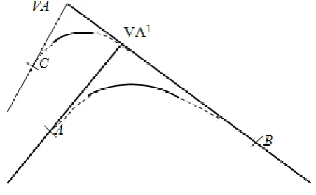
out that it already has a connection with some previous state C (Fig. 4), then the variants of AB and CB communication are compared on the objective function. The values of the objective function must correspond to the achievement of state B from the starting point of the route.

As a result for each new state B we record the state from which transition to it is possible and total value of the objective function (that is, from the beginning of the trace to state B) is minimal.

Figure 4. Comparison and rejection of options for transition to state B Such comparisons in state B may be made many times, whereas in the first step there was nothing to compare.

On completion of the described process, the construction of the last rotation angle is performed.

In this regard all states on all normals separated from the end point not further than Smax and no closer than Smin are consistently connected with the final state. If communication is possible, then the value of the objective function is calculated for it. If there are several such connections, they are compared by the total value of the objective function, and the best connection and value of the objective function are remembered. At the next step\, different initial states are at different distances from the end point of the route. If this distance is less than 2S min, we can connect initial state with the end point ofthe routeonly, otherwise one or more spline elements can be constructed. In the first case, all valid variants of the last element are considered and information about the best of them is stored.

In the second case, the next element is built and the process continues. It ends when all initial points of the next step can be connected with the end point of the route only. If several final states are specified, then these actions are performed sequentially for each of them. The best variant is remembered, and his connection with the previous state and the total value of the objective function are recorded.

As a result of the described algorithm work we will know the smallest total value of the objective function and all necessary information to restore the desired spline.

A reverse turn, starting from the final state, we successively consider links with previous states, that is, information recorded for each reachable state, including the communication address. We reach the connection with the initial state and form information about the spline for further use.

5. Results

The main result of the work done is a mathematical model of a special spline- approximation problem, when the number of elements is unknown, and there is a system of restrictions on the parameters of the desired spline. This model allowed to overcome the interconnection of adjacent curves and apply the method of dynamic programming. For this purpose, the above algorithm has been developed for the most difficult task of spline search with clothoids.

6. Discussion

The described algorithm, after simple simplifications, has been used to solve the problems of searching for splines, which do not have to satisfy the requirement of curvature continuity. In this case, there is no need for clothoids or any other elements of the transition curvature, which greatly simplified the task.

Programs have been developed for designing a plan and a longitudinal profile of the route. When computer-aided design of such objects, the "state of the system" was the beginning of the circle plus the direction of the tangent (side of the corner). After determining the VA and the angle of rotation for each new state, the radius of the circle is uniquely determined, since the intersection of the bisector and the normal towards the side of the angle at the transition point to the circle gives the center of the circle. All calculations are greatly simplified.

Additional simplifications are made in the program for designing a longitudinal profile by circular curves with tangential paths. In this case, the deviations of the original points from the spline were calculated by ordinates, and not by normals.

forming the search area. A multi-stage scheme usual for the application of dynamic programming is possible -the use of large discretes, then their reduction and the formation of a search area with the use of the obtained solution.

7. Conclusions

Existing spline - approximation programs are included in a new CAD system of a linear structure routing. Software implementation of the search for a spline with clothoid requires much more time. The work is currently suspended due to the lack of funding. First of all, this program is necessary to obtain an initial approximation for the existing optimization program of spline parameters using the nonlinear programming algorithm [1]. This program can use a more complex objective function and additional restrictions on the coordinates of individual points of the spline.

Currently, to calculate the initial approximation for this program, the user must determine the position of each tangential path. He can visualize the “chain” and mark two points on the screen on each tangential path, or visualize a corner diagram and mark one point on each horizontal section of the angle diagram. Further, the spline with clothoids is calculated automatically by a special program. The implementation of the algorithm described above will relieve the user from this work.

The advantages of computer-aided design, using optimization methods, before developing design solutions in an interactive mode will become obvious.

REFERENCES

[1] Struchenkov V. I., Methods to optimize the routes in the CAD systems of linear structures. Moscow, Solon – Press, 2014. 271 p.

[2] BentleyRailTrack]. URL: http://www.bentley.com/ Visited January 28, 2019.

[3] CARD/1 URL: http://www.card-1.com/en/home/ Visited January 27, 2019.

[4] Autodesk. .URL: https://www.architect-design.ru/autodesk /autocad/ Visited January 27, 2019.

[5] Credo-Dialog. URL: https://credo-dialogue.ru/Visited Janu ary 28, 2019.

[6] V. I. Struchenkov, Computer Technologies in Linear Structures Routing, Russian Technological Journal, 2017, vol 5, No 1, 28-41 pp.

[7] V. I. Struchenkov, Nonlinear Programming Algorithm for CAD Systems of Line Structure Routing, World Journal of Computer Application & Technology, 2014,vol. 2, No 5, 114-120 pp.

[8] J. H. Alberg, E. N. Nilson, J. L. Walsh the Theory of Splines

and Their Application. New York, Academic Press, 1967,316 p.

[9] Bellman R., Dynamic Programming. Princeton University Press, Princeton, New Jersey, 1957. 402 p.

[10] R. Bellman, S. Dreyfus, Applied Dynamic Programming. Princeton University Press, Princeton, New Jersey, 1962, 460 p.

i _{This research did not receive any specific grant from finding agencies in}