Optimal Unit Commitment with Ant Colony Algorithm

Optimal Unit Commitment with Ant Colony Algorithm

Majid Alizadeh Moghadam

*

_{, Hasan Keshavarz Ziyarani}

Electrical Engineering Department, University of Ghiaseddin Jamshid Kashani, Iran *Corresponding Author: [email protected]

Copyright © 2014 Horizon Research Publishing All rights reserved.

Abstract

This paper presents an improved ant colony search algorithm that is suitable for solving unit commitment (UC) problems. Ant colony algorithm (ACA) is a meta-heuristic technique for solving hard combinatorial optimization problems. It is a population-based approach that uses exploitation of positive feedback, distributed computation as well as constructive greedy heuristic. The ACA was inspired by the behavior of real ants that are capable of finding the shortest path from food sources to the nest without using visual cues. The constraints used in the solution of the UC problem using this approach are: real power balance, real power operating limits of generating units, spinning reserve, startup cost, and minimum up and down time constraints. The approach determines the units schedule followed by the consideration of unit transition related constraints. The proposed approach is expected to yield a better operational cost for the UC problem of production of 50 power plant units.

Keywords

Ant Colony Search Algorithm, Optimization, and Unit Commitment

1. Introduction

The unit commitment problem is a hard combinatorial mixed integer optimization problem to determine the optimum schedule of generating units while satisfying a set of system and unit constraints. Finding a good solution to the unit commitment problem in a reasonable time is very critical, since it could mean significant annual financial savings in power generating costs.

Several solution techniques have been applied to solve the problem. These include deterministic, meta-heuristic, and hybrid approaches. Deterministic approaches include the priority list method, dynamic programming, Lagrangian Relaxation (LR). The priority list is the simplest and fastest but achieves poor final solutions. The LR method provides a fast solution but it may suffer from numerical convergence and solution quality problems.

Due to the mixed binary and continuous variable nature, of the UC problem, traditional optimization techniques may miss the optimal solution. In addition, dimensionality of the

UC problem limits the application of traditional optimization techniques to small size system. Recently, meta-heuristic approaches became popular in the effort to overcome shortcomings of traditional optimization techniques. Techniques such as genetic algorithms, evolutionary programming, simulated annealing, and tabu search have been widely investigated to solve the UC problem. These methods can accommodate more complicated constraints and are claimed to produce solutions of improved quality.

The ACA is a meta-heuristic technique proposed to find a near optimal solution to the UC problem. The ACA was inspired by the behavior of real ants which are capable of finding the shortest path from food sources to the nest without using visual cues. The technique has been tested successfully on diverse complex combinatorial optimization problems. Also, it has been shown that the ant colony method performs with little variability over problem diversity or random number seed. In addition, the ACA introduces an entirely new solution at each iteration, while other meta-heuristic optimization techniques are based on improvement of the solution or set of solutions obtained from the previous iteration. During the solution process of the UC problem using the ACA, the obtained solution is always feasible. Moreover, the ACA does not require major assumptions and approximations that limit the solution space.

The paper is organized as follows: Section 2 contains the Unit Commitment problem formulation; Section 3 introduces the paradigm of the ACA and includes a discussion on its application to solve the UC problem; Section 4 presents the performance and discussion of running the algorithms to solve the UC problem; and conclusions are presented in Section 5.

2. Problem Formulation

The objective of the unit commitment problem is to determine the output level of units in each time stage that yield the minimum total cost while satisfying the problem constraints. The UC problem is described as follows:

Subject to:

, , , , ,1 , 1

( )T (1 )

ij ij ij ij ij ij j iN

Min J v FC P v v SC− = ∈

 

a)

Real power balance constraint

, , ,

ij ij Dj iN

v P P J T ∈

= ∈

∑

(2)

b) Real power operating limits of generating unit

min max

, , ,

,

;

ij i ij ij i

v P

≤

P v P J T i N

≤

∈

∈

(3)

c)

Spinning reserve constraint

, ,1

, ,1

(1 1), ;

1 ( 1 1), ;

ij ij up

ij d ij

v I x j j T i N

v I j x j T i N

−

−

≥ ≤ ≤ − ∈ ∈

≤ − − + ≤ ≤ − ∈ ∈ (4)

Where:

N: number of generating units, T : the total time horizon (hours),

, i j

P

_{: real power output of unit} i at stage j (MW), ,

i j

FC

: function representing the production cost of unit i where a0,i, a1,iand a2,iare the cost parameters:

2

, , 0, 1, , 2, ,

($ / ) : (

hr FC

_{i j i j}

P

)

=

a

_i

+

a P

_{i i j}

+

a P

_{i i j} (5)

j

PD : load at stage j(MW) ,

i j

v : control variable, with

, ₁0

i j if unit i is off at stage j v

if unit i is on at stage j

 =  

, res j

P : power reserve at stage j (MW), ( )

I x : logic function , 0 if x is false and 1 otherwise, ,

i j

x : the consecutive time unite i has been up (+) or down (-) (hrs) from the initial stage to stage j,

, i j

SC : the startup costs incurred during the transition of unit i from off to on during stage j

The system and unit capacity related constraints can be handled by solving the economic dispatch problem at each state. After the search space of multi-stage scheduling was determined, the unit transition related constraint and startup cost will be considered during the process of state transition by the ant colony search algorithm.

3. Ant Colony Behavior

The ant colony algorithm (ACA) mimics the behavior of real ants . It has been found suitable for solving UC problem that belong to a class of hard combinatorial optimization problems. The optimum paths followed by artificial ants (agents) are determined by their movements in a discrete time domain. While moving, agents lay some pheromone along their paths. Also, the agents are memory less. That is, regardless of the information acquired from their previous paths, the agents' decision to move from the present state r to the next state s is based on two measures. These are the length of the path which connects the present state to the next one, and the desirability measure (pheromone level). In brief, the paradigm of the ACA is such that each agent generates a

completed path (tour), by choosing the next states to move to according to a probabilistic state transition rule. This rule reflects the preference of agents to move on shorter paths that connect the current state to the next state and are also endowed with high level of pheromone.

In addition, while constructing its tour, an agent modifies the level of pheromone on the traversed paths by applying the local updating rule. The pheromone level on the traversed paths is lowered (evaporated) so that these paths become less attractive to other agents. This property gives agents a higher probability to explore different paths and find an improved solution. In other word, the role of the local updating rule is to make the desirability of paths change dynamically. This way, the agents can avoid being trapped in a local search based on the best previous tour.

Once all agents have reached the final state and have identified the best-tour-so-far based on the value of the objective function, they update the pheromone level on the paths that belong to the best tour by applying a global pheromone updating rule. This is intended to allocate a higher level of pheromone on the paths which belong to the best-tour-so-far. This rule is similar to a reinforcement learning scheme in which better solutions get a higher reinforcement. The rules that apply to agents while trying to find the best path solution are presented below.

3.1. State Transition Rule

Each agent builds a completed path to the end state, which occurs at the final stage. This takes place through the recurring application of the state transition rule. This rule calls for an agent located on state r at the current stage to move to state s at the next stage along a shorter path with a high amount of pheromone

𝜼𝜼

rs. This is achieved by a state transition rule that utilizes both the inverse of the length of the path

𝜼𝜼

rsand the amount of pheromone τrs.

In the UC problem, the transition cost from the present to the next hour TCrs, simulates the length of the path taken by an agent to reach the next state s from the current state r.

][

arg max

_{( )}

{[

] },

₀

if q q

ru ru

u J r

s

k

otherwise

q

t

h

s

   

≤

∈

=

(6)

u(k): a set of states in the next stage that can be visited by agent k positioned on state r

1

rs

TC

rs

h =

: the inverse of the transition cost

TCrs

with rs

being the path from state r at the current stage to state s at the next stage

rs

t

: the pheromone level on the path connecting state r to state s,

q

: a uniformly distributed random number in [0, 1],

0

σ: a random variable selected according to the probability distribution given by :

][

][

[

]

_{, if}

_(r)

[

]

,

_{( )}

0

rs rs

_{s Jk}

ru ru

Pk rs u J r

_k

otherwise

q

t h

q

t h

        

∈

∑

=

=

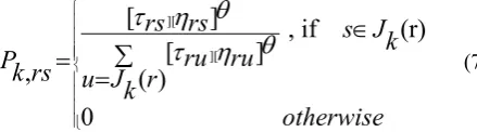
(7)

with θ being a parameter which determines the relative importance of pheromone versus path length (θ > 0).

The parameter q0 determines the relative importance of

choosing the more preferable (exploitation) versus less desirable (exploration) paths. Every time an agent in a current state r has to choose a next state s, it samples a random number

0

< <

q

1

. According to (1), ifq q≤ 0, the

best path is an exploitation one, otherwise an exploration path is chosen according to (1) and (2).

3.2. Local Updating

During the establishment of its path, an agent changes the pheromone level on the traversed path (local updating) by applying the local updating rule (3). This rule has the effect of lowering the pheromone level (evaporation) on the traversed paths so that these become less attractive to other agents.

(1

).

_{. 0}

rs

rs

t

= −

r t

+

r t

(8)

r

: decay/evaporation coefficient

(0

< <

r

1)

,

0

t

: initial pheromone level, ₀

1

J

t

=

where J is a rough approximation of the optimum value of the cost function .

Using the sum of the initial minimum transition costs to estimate J and keeping it throughout the solution process was found to be a good approach.

3.3. Global Updating

After all the agents have built their individual solutions, a global pheromone updating rule is applied only to the path that labeled the best-tour-so-far. It allocates a higher pheromone level to this tour. This is equivalent to a reinforcement learning scheme in which better solutions get a higher reinforcement. Global pheromone updating is performed by applying (9)

(1

).

.

rs

rs

rs

t

= −

α t

+ ∆

α t

(9)

*

1

( ) , if (r,s) global-best tour

0 otherwise

J

rs

t





−

_∈

∆

=

(10)

α

: pheromone decay parameter (0 <

α

< 1)

J* : the best value of the objective function reached so far.

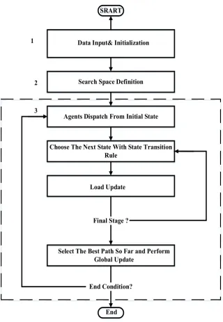
[image:3.595.73.293.111.172.2]

4. Ant Colony Algorithm

Figure 1 illustrates the computational flow of the ACA to solve the unit commitment problem. The main computational processes for the traditional ACA are discussed as follows

Step 1. Initialization

i. Setup the parameters (q0, θ, α, ..., etc) and capture the system data (load, reserve, minimum up and down time, and different cost components).

ii. Build the unit status table.

Step 2. Search space definition and economic dispatch

i. Establishing the multi-stage search space. All the possible permutations form this search space. ii. Economic dispatch

Step 3. The ACA cycle

i. Place the agents at the initial state.

ii. Select the next state that each agent will move to by applying the state transition rules (7) and (8). iii. Update the local pheromone levels using (9). iv. Update the cost functions for each path

considering the transition cost.

v. When all agents have reached the final stage (i.e., each has generated a completed path or tour), apply the global updating rule (10) to the best-tour-so-far.

vi. One full cycle is now completed. The process ends if no or minor improvement in the objective function value is observed; otherwise steps i-vi are repeated.

In the ACA as described above, all agents are moving together from the initial stage to the final stage. The pheromone level is updated locally after all agents move from one stage to the other. In the proposed ACA, one agent moves at a time from the initial to the final stage. During the movement of each agent the pheromone level is updated locally. Moving one agent at a time will give all the other agents the opportunity to exploit the experience of the previous agents. For example, in the first cycle of the solution of unit commitment problems, all agents start with same initial pheromone level (in this problem this value is taken 0.01). The first agent will move from the initial stage to the final stage. Movement decision is based on the initial pheromone level and the transition cost. During the movement of the first agent the pheromone level for the selected path by the agent will be updated. Now, when the second agent moves from the initial to the final stage, it uses the information (pheromone level)

SRART

Final Stage ?

End Condition? Data Input& Initialization

Search Space Definition

Agents Dispatch From Initial State

Choose The Next State With State Transition Rule

Load Update

Select The Best Path So Far and Perform Global Update

End 1

2

[image:4.595.145.466.74.538.2]

3

Figure 1. Algorithm of problem solving

5. Results

In this section we present the results. We have attempted to compare the results in different states to obtain a better view about solving the problem.

5.1. Production Cost

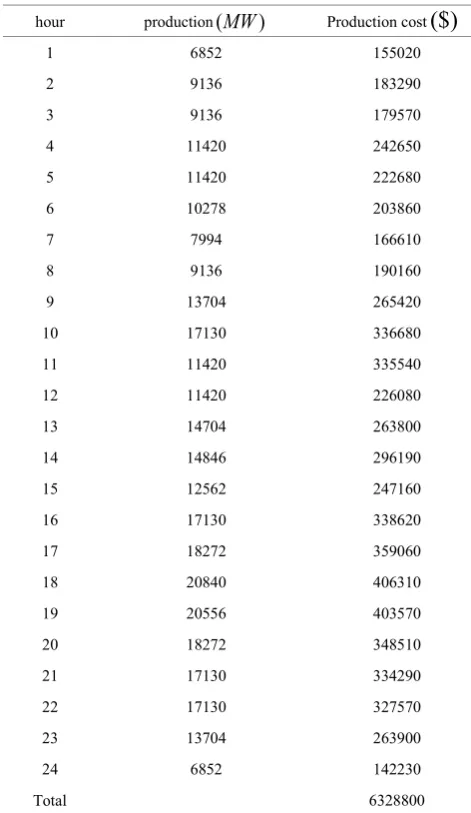
Following running the program, production planning is implemented for a time period of 24 hours through ant colony algorithm. In general, production rate of each unit, data of unit hourly, which should be placed into the power system and production cost, are expected to be the optimum output of an exploitation planning. Table 1 demonstrates the hourly production and its cost. As it is shown, cost has a direct relationship with production so with the production

increase the cost also increase. However, production increase is not the sole factor through the exploitation planning process, and exploitation constraints and power plants constraint will also cause cost raise. The total exploitation cost of units in 24 hours equals 6328800 dollars. This cost includes the transient and fixed cost of power plants and the extra cost imposed by the constraints to the system.

5.2. The Effect of Number of Agents (ants)

[image:5.595.312.552.90.275.2]

this section we will see this is not the case. In this section within two scenarios the production cost for the first hour has been calculated, one in which the number of agents is 25 being under 50 agents for the main problem solution and the other in which the number of agents is 100 , being over the number of problem solving agents.

Table 1. Amount & cost of production by hour

Production cost

($)

production

(

MW

)

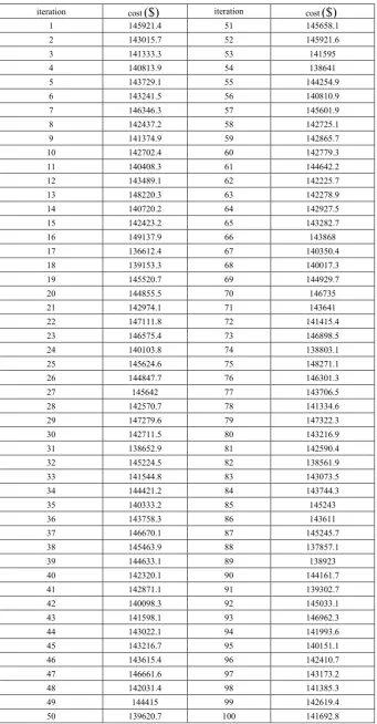
hour 155020 6852 1 183290 9136 2 179570 9136 3 242650 11420 4 222680 11420 5 203860 10278 6 166610 7994 7 190160 9136 8 265420 13704 9 336680 17130 10 335540 11420 11 226080 11420 12 263800 14704 13 296190 14846 14 247160 12562 15 338620 17130 16 359060 18272 17 406310 20840 18 403570 20556 19 348510 18272 20 334290 17130 21 327570 17130 22 263900 13704 23 142230 6852 24 6328800 Total

5.2.1. The First Scenario: The Number of agents 25

Twenty five agents have been utilized to search the problem space. As shown in table 2, the best answer lies in the 4th _{iteration and equals 141016.1 MW ,which is higher}

by 2.97% compared to the best problem solving result with 50 agents (136822.7 MW), showing the error of 2.97% regarding a more accurate answer to the problem . Thus, if the number of agents is under usual rate, the possibility of error incidence will increase.

Table 2. Production costs by hour for 25 agents

cost

($)

iteration cost

($)

Iteration 144629.1 14 146769.2 1 145029.7 15 148321.3 2 141936.4 16 142222.7 3 146678.2 17 141016.1 4 141761.5 18 144982.1 5 146434.2 19 145061.6 6 140322.4 20 142156 7 146034.3 21 142287 8 144710.7 22 146359.9 9 145377.4 23 143798.1 10 146316.6 24 142654.2 11 144629.1 25 143568 12 143097.5 13

5.2.3. The Problem of Local Optimization and Lack of Convergence

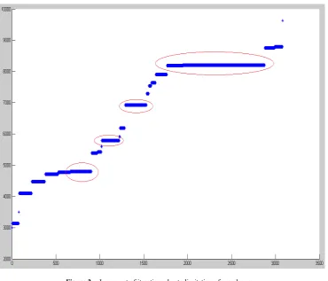
The use of meta-heuristic methods to solve a problem increases the probability of lack of convergence and trapping in local optimization. As stated, one of the methods to prevent this problem is to cause excitation in search space of the agents. In this project this method is used to solve the problem of local optimization and lack of convergence of algorithm. In most cases, of course, after frequent iterations convergence acquired, However, in this case the answer is either local optimization or a long period of time is required to receive the answer due to the iteration increment. Figure 2 indicates an example of the increase in the number of iterations due to the search space limitation. In this chart, total units production power is plotted in terms of different iterations. It can be observed that following 3081 iterations optimum answer has been obtained. As demonstrated in the figure, the red circles indicate trapping in non-convergent iterations in which the number of iterations reaches 1000, causing elongation of production planning process.

[image:5.595.57.293.174.581.2]

[image:6.595.135.477.89.744.2]

[image:7.595.122.493.75.392.2] [image:7.595.121.489.395.706.2]

Figure 2. Increment of iterations due to limitation of search space

6. Conclusions

This paper deals with the unit commitment problem using ant colony algorithm. To solve this problem two scenarios were taken into account in the first place. The first scenario was choosing 25 agents (ants) and the second scenario was choosing 100 agents. The results of the two scenarios were compared with each other, and ultimately 50 agents was determined which seems a more reasonable number and the results cover a wide range of search space. The results obtained from ant’s colony algorithm to solve the problem of unit commitment indicates the efficiency of this algorithm in solving the problem.

REFERENCES

[1] M. Y. El-Sharkh, N. S. Sisworahardjo, A. Rahman, M. S. Alam, “An Improved Ant Colony Search Algorithm for Unit Commitment Application,” IEEE PSCE, 2006.

[2] N.S.Sisworahardjo, A. A. EL-Keib, “Unit Commitment Using the Ant Colony Search Algorithm,” IEEE. Large Engineering Systems conference on Power Engineering, 2002.

[3] A. J. Wood and B. F. Wollenberg, “Power generation operation and control,” 2”d Ed., John Wiley and Sons, New York, 1996.

[4] C. K. Pang and H. C. Chen, “Optimal short-term thermal unit commitment,” IEEE Transaction on Poiver Systems, PAS-95, pp. 1336-1341, 1976.

[5] S. J. Wang, S. M. Shahidehpour, D. S. Kirschen, I. S. Mokhtar, and G.D. Irisarri, “Short-term generation scheduling with transmission and environmental constraints using an augmented Lagrangian relaxation,”IEEE Transactions on Power Systems, vol. 10, no.3, pp. 1294-1301, Aug. 1995. [6] M. Aizadeh. Moghadam, S. Jalilzadeh, “Control of AGC in

Interconnected Power System with Diverse Sources of Power Generation” Universal Journal of Electrical and Electronic Engineering, vol. 2, no. 7, pp. 259-269, 2014.

[7] R. H. Lasseter, A. Akhil, C. Marnay, J. Stephens, J. Dagle, R. Guttromson, A. Meliopoulous, R. Yinger, and J. Eto, The CERTS Microgrid Concept,white paper for Transmission Reliability Program,Office of Power Technologies, U.S. Department of Energy, Apr. 2002.

[8] P. Piagi and R. H. Lasseter, “Autonomous control of microgrids,” in Proc. IEEE Power Eng. Soc. General Meeting, 2006, 2006, 8 pp.

[9] M. C. Chandorkar, D. M. Divan, and R. Adapa, “Control of parallel connected inverters in standalone AC supply systems,” IEEE Trans. Ind. Appl., vol. 29, no. 1, pp. 136–143, Jan./Feb. 1993.