Voltage stabilizer of generator output through field current control using fuzzy logic

VOLTAGE STABILIZER OF GENERATOR OUTPUT THROUGH FIELD CURRENT CONTROL USING FUZZY LOGIC

CLARA VALDEZ

A project report submitted in partial

Fulfillment of the requirement for the award of the Degree of Master of Electrical & Electronic Engineering

Faculty of Electrical & Electronic Engineering Universiti Tun Hussien Onn Malaysia

ABSTRACT

ABSTRAK

TABLE OF CONTENTS

THESIS STATUS APPROVAL EXAMINERS’ DECLARATION TITLE

DECLARATION ii

ACKNOWLEDGEMENT iii

ABSTRACT iv

ABSTRAK v

CONTENTS vi

LIST OF TABLES ix

LIST OF FIGURES x

LIST OF SYMBOLS AND ABBREVIATIONS xii

CHAPTER 1 INTRODUCTION 1

1.1 Project Background 1

1.2 Problem Statements 2

1.3 Project Objectives 2

CHAPTER 2 LITERATURE REVIEW 4

2.0 Introduction 4

2.1 Fuzzy Logic 7

2.1.1 A Comparison of Classical Set and Fuzzy Set 8

2.2 Practical relevance of fuzzy modelling 11

2.2.1 Fuzzy Sets with a Continuous Universe 13

2.3 Fuzzy Set-Theoretic Operations 14

2.3.1 Containment or Subset 15

2.3.2 Union (Disjunction) 15

2.3.3 Intersection (Conjunction) 16

2.3.4 Complement (Negation) 17

2.4 Rule-Based Fuzzy Models 18

2.5 Electric Generator 18

2.5.1 Principles of Electric Generator 20

2.6 Voltage Regulator 22

CHAPTER 3 PROJECT DEVELOPMENT 25

3.1 Formulating Membership Functions 25

3.2 Membership Functions in Fuzzy Logic Toolbox Software 27

3.3 Fuzzy Logic Controller 33

3.3.1 Application Areas of Fuzzy Logic Controllers 33

3.4 Components of FLC 34

3.4.1 Fuzzification Block or Fuzzifier 34

3.4.3 Defuzzification Block or Defuzzifier 36

CHAPTER 4 METHODOLOGY 39

4.1 Fuzzy Logic Controller Design 39

4.2 Membership Function Design 40

4.3 Output Linguistic Variable 43

4.3.1 Rule Base Design for the Output 44

4.4 Variable Of Fuzzy Logic Control 45

4.5 Design of the Fuzzy Logic Controller using MATLAB 47

4.6 MATLAB Simulation 60

CHAPTER 5 RESULT, ANALYSIS AND DISCUSSION 62

5.1 Simulation Results 62

5.2 Analysis 64

5.3 Discussion 68

CHAPTER 6 CONCLUSION, DISCUSSION AND RECOMMENDATION 70

6.1 Conclusion 70

6.2 Recommendation 71

LIST OF TABLES

Table2.1: Different modelling paradigms. 7

Table 4.1: Fuzzy sets and the respective membership functions for voltage (v) 41

Table 4.2: Fuzzy sets and the respective membership functions for Change

in voltage (∆v) or derivative rate of change of voltage. 42

Table 4.3: Fuzzy sets and the respective membership functions for

Output voltage (ω_{sl) 43}

LIST OF FIGURES

Figure 2.1: Example of Classical Set and Fuzzy set 8

Figure 2.2: Evaluation of a crisp, interval and fuzzy function for crisp, interval and

fuzzy arguments 10

Figure 2.3: Membership Function on a Continuous Universe 13

Figure 2.4: Operations on Fuzzy sets - The concept of containment or subset 15

Figure 2.5: Operations on Fuzzy sets - Two Fuzzy sets A and B 16

Figure 2.6: Operations on Fuzzy sets - A B 17

Figure 2.7: Operations on Fuzzy sets - Fuzzy set A and its Complement Ā 17

Figure 2.8: Electric Generator 19

Figure 2.9: Two Types of Rotor Construction 22

Figure 3.1: Examples of four classes of parameterized MFs 26

Figure 3.2: Triangular & Trapezoidal Membership functions 29

Figure 3.3: Gaussian distribution curve 30

Figure 3.4: Sigmoidal MFs 31

Figure 3.5: Z, S, and Pi MFs 32

Figure 3.7: Various Defuzzification schemes for obtaining crisp outputs 38

Figure 4.1: Block Diagram of Variables of the Fuzzy Logic Controller 45

Figure 4.2: Flow Chart for the Fuzzy Logic-Based Generator controller 46

Figure 4.3: FIS editor window in MATLAB 55

Figure 4.4: FIS editor: rules window in MATLAB 56

Figure 4.5: Membership function for the input Voltage (v) 57

Figure 4.6: Membership function for the input Change in Voltage (∆v) 58

Figure 4.7: Membership function for the output Change of voltage 59

Figure 4.8:Voltage Stabilizer of Generator using Fuzzy Logic Model

in SIMULINK 60

Figure 5.1: Voltage output (regulated) 63

Figure 5.2: Voltage output with voltage reference 64

Figure 5.3: Three dimensional plot of the control surface 65

Figure 5.4: Rule viewer for Output viewer with inputs v = 0 and ∆v = 0 66

LIST OF SYMBOLS AND ABBREVIATIONS

element of

Mu

union

intersection

increment

greater than

alpha

beta

COA Centroid of Area

BOA Bisector of Area

MOM Mean of Maximum

SOM Smallest of Minimum

LOM Largest of Maximum

AC alternating current

TS Takagi–Sugeno

MFs membership functions

FLC Fuzzy Logic Control

Vref voltage reference

PL Positive Large

PM Positive Medium

PS Positive Small NL Negative Large

NM Negative Medium

NS Negative Small

ZE Zero

CHAPTER 1

INTRODUCTION

1.1 Project Background

1.2 Problem Statements

A number of research studies on the design of the excitation controller of synchronous generator have been successfully carried out in order to improve the damping characteristics of a power system over a wide range of operating points and to enhance the dynamic stability of power systems. When the load is changing, the operation point of a power system will be varies. When there is a large disturbance, there are considerable changes in the operating conditions of the power system. Therefore, it is impossible to obtain optimal operating conditions through a fixed excitation controller. To overcome this problem in this project is designed a voltage stabilizer of generator output through its field current control by applying a Fuzzy Logic Controller.

1.3 Project Objectives

The major objectives of this research are:

a) To derive the generator model based on field current control.

1.4 Project Scopes

The scopes of this project are:

a) Type of generator going to studied is an AC Generator. b) The model is based on field current model.

c) The controller apply is Fuzzy Logic

CHAPTER 2

LITERATURE REVIEW

2.0 Introduction

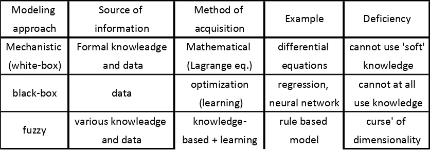
Developing mathematical models of real systems is a central topic in many disciplines of engineering and science. Models can be used for simulations, analysis of the system’s behaviour, better understanding of the underlying mechanisms in the system, design of new processes, or design of controllers.

Traditionally, modelling is seen as a conjunction of a thorough understanding of the system’s nature and behaviour, and of a suitable mathematical treatment that leads to a usable model.

Difficulties encountered in conventional “white-box” modeling can arise, for

instance, from poor understanding of the underlying phenomena, inaccurate values of

various process parameters, or from the complexity of the resulting model. A complete

understanding of the underlying mechanisms is virtually impossible for a majority of real

systems. However, gathering an acceptable degree of knowledge needed for physical

modeling may be a very difficult, time-consuming and expensive or even impossible task.

Even if the structure of the model is determined, a major problem of obtaining accurate

values for the parameters remains. It is the task of system identification to estimate the

parameters from data measured on the system. Identification methods are currently

developed to a mature level for linear systems only. Most real processes are, however,

nonlinear and can be approximated by linear models only locally.

A different approach assumes that the process under study can be approximated by using some sufficiently general “black-box” structure used as a general function approximated. The modelling problem then reduces to postulating an appropriate structure of the approximated, in order to correctly capture the dynamics and nonlinearity of the system. In black-box modelling, the structure of the model is hardly related to the structure of the real system.

that the known parts of the system are modeled using physical knowledge, and the unknown or less certain parts are approximated in a black-box manner, using process data and black-box modeling structures with suitable approximation properties. These methods are often denoted as hybrid, semi-mechanistic or “gray-box” modeling.

Modeling Source of Method of

approach information acquisition

Mechanistic Formal knowleadge Mathematical differential cannot use 'soft'

(white-box) and data (Lagrange eq.) equations knowledge

optimization regression, cannot at all

(learning) neural network use knowledge

various knowleadge knowledge- rule based curse' of

and data based + learning model dimensionality Example Deficiency

black-box

fuzzy

data

Table 2.1: Different modelling paradigms.

2.1. Fuzzy Logic

Fuzzy Logic was initiated in 1965 [2] by Lotfi A. Zadeh, professor for computer science at the University of California in Berkeley. Basically, Fuzzy Logic (FL) is a multi-valued logic that allows intermediate values to be defined between conventional evaluations like true/false, yes/no, high/low and more. Notions like rather tall or very fast can be formulated mathematically and processed by computers, in order to apply a more human-like way of thinking in the programming of computers [3].

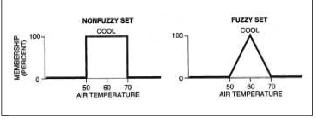
2.1.1 A Comparison of Classical Set and Fuzzy Set

Let X be a space of objects (called universe of discourse or universal set) and x be a generic element of X.

A classical set A (A is a subset of X) is defined as a collection of elements or objects x X, such that each x can either belong or not belong to the set A. By defining a characteristic function for each element in X, the classical set A by a set of ordered pairs (x,0 ) or (x,1 ) can represented which indicates x or x A, respectively.

Figure 2.1: Example of Classical Set and Fuzzy set

In spite of being an important tool for the engineering sciences, classical sets fail to replicate the nature of human conceptions, which tend to be abstract and vague. A fuzzy set [4] conveys the degree to which an element belongs to a set. In other words, if X is a collection of objects denoted generically by x, then a fuzzy set A in X is defined as a set of ordered pairs as below:

Where µA(x) is known as the membership function for the fuzzy set A. MF serves the purpose of mapping each element of X to a membership grade (or membership value) between 0 and 1.Clearly, if the value of µA(x) is restricted to either 0 or 1, then A is reduced to a classical set and µA(x) is the characteristic function of A.

Fuzzy systems can be regarded as a generalization of interval-valued systems, which are in turn a generalization of crisp systems. This is depicted in Figure2.2 which gives an example of a function and its interval and fuzzy forms. The evaluation of the function for crisp, interval and fuzzy data is schematically depicted as well. Note that a function can be regarded as a subset of the Cartesian product X x Y, as a relation. The evaluation of the function for a given input proceeds in three steps:

i. Extend the given input into the product space Y (vertical dashed lines in Figure 2. 2),

ii. Find the intersection of this extension with the relation,

iii. Project this intersection onto Y (horizontal dashed lines in Figure 2.2).

Figure 2.2: Evaluation of a crisp, interval and fuzzy function for crisp, interval and fuzzy arguments

2.2 Practical relevance of fuzzy modelling

1. Incomplete or vague knowledge about systems

Conventional system theory relies on crisp mathematical models of systems, such as algebraic and differential or difference equations. For some systems, such as electro-mechanical systems, mathematical models can be obtained. This is because the physical laws governing the systems are well understood. For a large number of practical problems, however, the gathering of an acceptable degree of knowledge needed for physical modelling is a difficult, time-consuming and expensive or even impossible task.

2. Adequate processing of imprecise information.

Precise numerical computation with conventional mathematical models only makes sense when the parameters and input data are accurately known. As this is often not the case, a modelling framework is needed which can adequately process not only the given data, but also the associated uncertainty. The stochastic approach is a traditional way of dealing with uncertainty. However, it has been recognized that not all types of uncertainty can be dealt with within the stochastic framework. Various alternative approaches have been proposed [7], fuzzy logic and set theory being one of them.

3. Transparent (gray-box) modelling and identification.

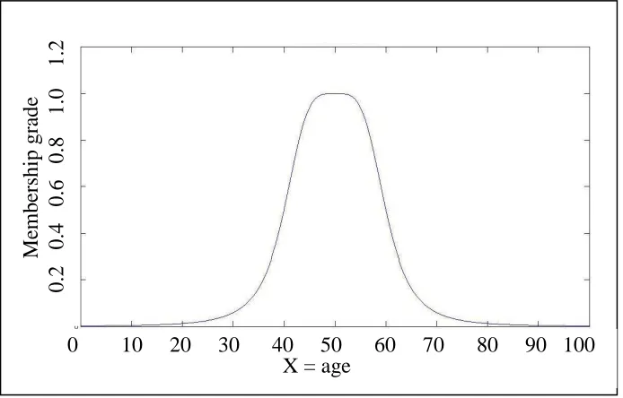
2.2.1 Fuzzy Sets with a Continuous Universe

Figure 2.3: Membership Function on a Continuous Universe

Let X be the set of possible ages for human beings. Then the fuzzy set A = “about 50 years old” may be expressed as

A

(x))|x

Where,

A

The aforementioned example clearly expresses the dependence of the construction of a fuzzy set on two things:

i. Identifying a suitable universe of discourse. ii. Laying down a suitable membership function.

M em b er sh ip g ra d e 0 .2 0 .4 0 .6 0 .8 1 .0 1 .2

0 10 20 30 40 50 60 70 80 90 100 X = age

(x) = ___1___ (x – 50)4

_{1 +}

At this point, it is imperative to state that the specification of membership functions is subjective; meaning that membership functions stated for the same notion by different persons will tend to vary noticeably. Subjectivity and non-randomness differentiate the study of fuzzy sets from probability theory.

I. Crisp variable: A crisp variable is a physical variable that can be measured through instruments and can be assigned a crisp or discrete value, such as a temperature of 30 0_{Celsius, an output voltage of 8.55 Volt etc.}

II. Linguistic variable: When the universe of discourse is a continuous space, the common practice is to partition X into several fuzzy sets whose MFs cover X in a more or less uniform manner. These fuzzy sets, which usually carry names that conform to adjectives appearing in our daily linguistic usage, such as “large”, “medium” or “small”, are called linguistic values. Consequently, the universe of discourse X is often called the linguistic variable.

2.3 Fuzzy Set-Theoretic Operations

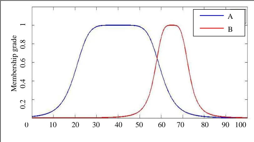
2.3.1 Containment or Subset

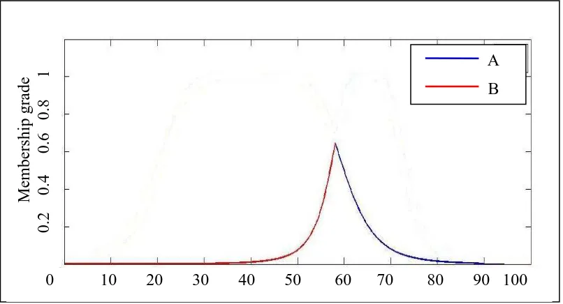
Fuzzy set A is contained in fuzzy set B (or, equivalently, A is a subset of B) iff µA B (x) for all x. The following figure clarifies this concept.

Figure 2.4: Operations on Fuzzy sets - The concept of containment or subset

2.3.2 Union (Disjunction)

The union of two fuzzy sets A and B is a fuzzy set C, written as , whose MF is related to those of A and B by

µc(x) = max (µA(x), µB(x)) = µA(x) µB(x) (2.4) 0 10 20 30 40 50 60 70 80 90 100

Equivalently, union is the smallest fuzzy set containing both A and B. Then again, if D is any fuzzy set encompassing both A and B, then it also contains

Figure 2.5: Operations on Fuzzy sets - Two Fuzzy sets A and B

2.3.3 Intersection (Conjunction)

The intersection of two fuzzy sets A and B is a fuzzy set C, written

as whose MF is related to those of A and B by

µc(x) = min (µA(x), µB(x)) = µA(x) µB(x) (2.5) Analogous to the definition of union, intersection of A and B is the largest fuzzy set which is contained in both A and B.

0 10 20 30 40 50 60 70 80 90 100

Figure 2.6: Operations on Fuzzy sets - A B

2.3.4 Complement (Negation)

The complement of fuzzy set A, designated by _Ā ( ¬A, NOT A), is defined

as: µA(x) = 1- µA(x) .

(2.5)

Figure 2.7: Operations on Fuzzy sets - Fuzzy set A and its Complement _Ā 0 10 20 30 40 50 60 70 80 90 100

M em b er sh ip g ra d e 0 .2 0 .4 0 .6 0 .8 1 A B M em b er sh ip ( P er ce n t) 5 0 1 0 0

NOT COOL COOL NOT COOL

2.4 Rule-Based Fuzzy Models

In rule-based fuzzy systems, the relationships between variables are represented by means of fuzzy if–then rules of the following general form:

If antecedent proposition then consequent proposition:

The antecedent proposition is always a fuzzy proposition of the type “ is A” where is a linguistic variable and A is a linguistic constant (term). The proposition’s truth value (a real number between zero and one) depends on the degree of match (similarity) between and A. Depending on the form of the consequent two main types of rule-based fuzzy models are distinguished:

i. Linguistic fuzzy model: both the antecedent and the consequent are fuzzy propositions.

ii. Takagi–Sugeno (TS) fuzzy model: the antecedent is a fuzzy proposition; the consequent is a crisp function.

2.5 Electric Generator

An electric generator is a device used to convert mechanical energy into

induction" discovered in 1831 by Michael Faraday, a British scientist. Faraday discovered that the above flow of electric charges could be induced by moving an electrical conductor, such as a wire that contains electric charges, in a magnetic field. This movement creates a voltage difference between the two ends of the wire or electrical conductor, which in turn causes the electric charges to flow, thus generating electric current.

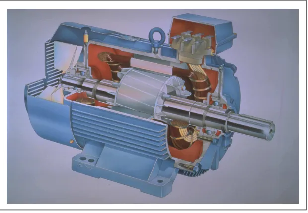
Figure 2.8: Electric Generator

The common type of electric generator, such as a bicycle dynamo, uses the

principle of electromagnetic induction to convert mechanical energy into electrical

energy. These devices carry one or more coils surrounded by a magnetic field,

typically supplied by a permanent magnet or electromagnet. In a direct current (DC)

generator, a mechanical switch (or Commutator) causes the rotor current to reverse

every half an electrical cycle so that the output current remains unidirectional. In an

alternating current (AC) generator, the rotor is driven by a turbine and electric

stations are of this type and they provide the electric power for general transmission

and distribution.

It must be turned by a prime mover which can be an internal combustion engine - driven, usually, by diesel oil or gasoline or can be a turbine, driven either by superheated steam or by hydro-electric power generation.

Generators are useful appliances that supply electrical power during a power outage and prevent discontinuity of daily activities or disruption of business operations. Generators are available in different electrical and physical configurations for use in different applications. For example, to produce dc power from an ac service or to produce 3-phase ac power from a single-phase ac service.

2.5.1 Principles of Electric Generator

The operation of a generator is based on Faraday’s law of electromagnetic induction. If a coil or winding is linked to a varying magnetic field, then electromotive force or voltage is induced across the coil. Thus, a generator has two essential parts: one that creates a magnetic field and the other where the energy is induced. The magnetic field is typically generated by electromagnets.

current conducted to it by means of carbon brushes bearing on slip rings or collector rings.

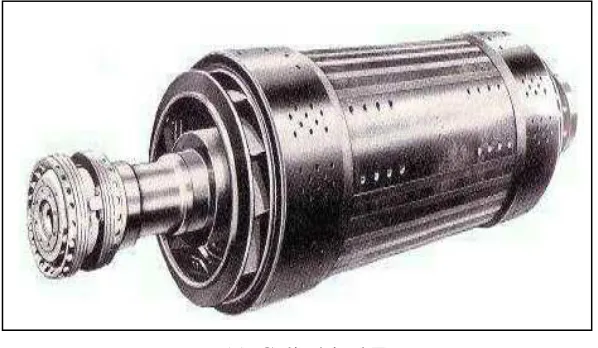
The rotor of the synchronous generator may be cylindrical or salient construction. The cylindrical type of rotor has one distributed winding and a uniform air gap. These generators are driven by steam turbines and are designed for high speed 3000 or 1500 r.p.m (two and four pole machines respectively) operation. The rotor of these generators has a relatively large axial length and small diameter to limit the centrifugal forces.

(a) Cylindrical Type

(b) Salient Type

Figure 2.9: Two Types of Rotor Construction: Source: Hubret,C. (1991)

2.6 Voltage Regulator

is required to keep the voltage constant, even when affected by these disturbing factors. Power system operation considered so far was under condition of steady load. However, both active and reactive power demands are never steady and they continually change with the rising or falling trend.

The voltage regulator may be manually or automatically controlled. The voltage can be regulated manually by tap-changing switches, a variable auto transformer, and an induction regulator. In manual control, the output voltage is sensed with a voltmeter connected at the output; the decision and correcting operation is made by a human being. The manual control may not always be feasible due to various factors and the accuracy, which can be obtained, depending on the degree of instrument and giving much better performance so far as stability.

In modern large interconnected system, manual regulation is not feasible and therefore automatic generation and voltage regulation equipment is installed on each generator. Automatic Voltage Regulator (AVR) may be discontinuous or continuous type. The discontinuous control type is simpler than the continuous type but it has a dead zone where no single is given. Therefore, its response time is longer and less accurate. Modern static continuous type automatic voltage regulator has the advantage of providing extremely fast response times and high field ceiling voltages for forcing rapid changes in the generator terminal voltage during system faults. Electronic control circuit is now used for the field control circuit as the closed loop system to obtain stable output voltage. Electronic control circuit is simple but the simple is the best. By using this control circuit for the system, the system cost is decreased and system reliability and design flexibility are increased.

electronic components. Depending on the design, it may be used to regulate one or more AC or DC voltages.

Electronic voltage regulators are found in devices such as computer power supplies where they stabilize the DC voltages used by the processor and other elements. In automobile alternators and central power station generator plants, voltage regulators control the output of the plant. In an electric power distribution system, voltage regulators may be installed at a substation or along distribution lines so that all customers receive steady voltage independent of how much power is drawn from the line.

There are numerous types of voltage regulators. These include positive voltage regulators, which are used to convert positive supply voltages to different positive voltage levels. There are also negative voltage regulators, which are used to convert negative voltage levels to different negative voltage levels. Additionally there are fixed and adjustable voltage regulators. Fixed voltage regulators will only produce a specific voltage out for a given input voltage values. Adjustable voltage regulators permit the output voltage of a regulator to be changed. This is often done by connecting a variable resistor to the voltage regulator.

REFERENCES

[1] Byung Ha Lee and Kwang Y. Lee( February 1991), "Dynamic and static voltage

stability enhancement of power systems," vol. 8, pp. 231- 238, IEEE Trans. Power

Systems.

[2] L.A. Zadeh (1965), Fuzzy Sets, Information and Control

[3] L.A. Zadeh, ”Making computers think like people,” IEEE. Spectrum, 8/1984,

pp. 26-32.

[4] L. A. Zadeh, “Fuzzy sets,” Information and Control, vol. 8, pp. 338-353, 1965.

[5] Pedrycz (1994); Yager and Filev.

[6] (Buchanan and Shortliffe, 1984; Patterson, 1990)

[7] (Smets, et al., 1988)

[8] ](Ljung, 1987)

[9] (Kosko, 1994; Wang, 1994; Zeng and Singh, 1995)

[11] Myinzu Htay and Kyaw San Win (2008), ‘Design and Construction of Automatic

Voltage Regulator for Diesel Engine Type Stand-alone Synchronous Generator’,

World Academy of Science, Engineering and Technolog

[12] J.-S. R. Jang, C.-T. Sun, E. Mizutani (1997), “Neuro-Fuzzy and Soft Computing,”

Pearson Education Pte. Ltd., ISBN 81-297-0324-6, chap. 2, chap. 3, chap. 4.

[13] http://www.mathworks.com/help/fuzzy/foundations-of-fuzzy-logic.html#bp78l70-2

[14] Ramón C. Oros, Guillermo O. Forte, Luis Canali, “Scalar Speed Control of a d-q Induction Motor Model Using Fuzzy Logic Controller”, Departamento de

Electrónica, Facultad Regional Córdoba, Universidad Tecnológica Nacional, Conf. paper.

[15] R.Ouiguini, K. Djeffal, A.Oussedik and R. Megartsi, “Speed Control of an

Induction Motor using the Fuzzy logic approach.”, ISIE’97 - Guimariies, Portugal, IEEE Catalog Number: 97TH8280, vol.3, pg. 1168 – 1172.

[15] J.-S. R. Jang, C.-T. Sun, E. Mizutani, “Neuro-Fuzzy and Soft Computing,” Pearson Education Pte. Ltd., ISBN 81-297-0324-6, 1997, chap. 2, chap. 3, chap. 4.