Comparison of impedance analysis and field analysis in eddy current testing

Journal of Chemical and Pharmaceutical Research, 2014, 6(2):178-186

Research Article

_{CODEN(USA) : JCPRC5}

ISSN : 0975-7384

Comparison of impedance analysis and field analysis in eddy current testing

Bo Ye*, Ming Li, Fei Chen, Fang Zeng, Zhangzhou He, Leilei Li and Ke Sun

Engineering Research Center of Smart Grid, Yunnan Province, Faculty of Electric Power

Engineering, Kunming University of Science and Technology, Kunming, China

_____________________________________________________________________________________________

ABSTRACT

This paper presents the theoretical basis of eddy current testing. Firstly, it introduces the impedance analysis method used in the field of eddy current testing. Then we analyze the skin effect and the phase lag on that basis. Next we introduce the field analysis method in eddy current testing. This article takes the Maxwell’s equations of time-harmonic electromagnetic field as a starting point and then describes both the equations and their boundary value problems with vector magnetic potential, and it studies the perturbed magnetic field caused by ideal defects on that basis. Finally, this paper analyzes and contrasts the impedance analysis method and the field analysis method in depth.

Key words: Eddy current; nondestructive testing; impedance analysis; field analysis

_____________________________________________________________________________________________

INTRODUCTION

Eddy Current Testing (ECT) [1-3] is a new non-destructive testing technology, which is based on Faraday’s law of electromagnetic induction and Maxwell’s equations [4-6]. In the process of ECT, when the coil with sinusoidal alternating current closes to the measured conductor, the electromagnetic induction occurs due to the interaction between the excitation electromagnetic field generated by coil and the measured conductor. The eddy current interlinks the excitation electromagnetic field induces in external and internal layers of a test piece. Meanwhile, the eddy current engenders corresponding alternating electromagnetic field as well and reacts upon the original magnetic field, therefore, the internal electromagnetic field of coils changes. Along with the exciting electromagnetic field changing more and more quickly, the induced electromotive force external and internal the conductor increases and so does the induced eddy current. There are many influencing factors on eddy current as well as the methods to analyze eddy current testing signal. This paper mainly discusses two common analysis methods in the field of eddy current testing: the impedance analysis method and the field analysis method, and makes analysis and contrast on the two methods in detail, which lays a solid theoretical foundation in the research in subsequent chapter.

EDDY CURRENT TESTING BASED ON IMPEDANCE ANALYSIS

In the field of ECT, detection signal comes from the variation of detecting coil impedance or the changes of secondary coil’s induced voltage. As there are many factors affect impedance and voltage and influence degree by these factors are different, there must have the means and methods to eliminate interference factors of extracting a meaningful signal for achieving the purpose of eliminating interference signal. There are many means and methods to eliminate interference factors during the development process of eddy current testing, whereas the ECT technology does not make a significant breakthrough nor achieve wide applications until Dr. Forster brought impedance analysis into it [7-10].

______________________________________________________________________________

(1) COIL IMPEDANCE

The probe coil of eddy current testing is the key to ECT system, and it is wound by metal wires. Probe coil not only has inductance, but also has resistance and capacitance. Therefore, the coil can be represented by a series circuit of inductors, capacitors and resistors, while it may usually ignore the distributed capacitance between turns. The complex impedance of coil itself can be expressed in the following equation:

Z= +R j Lω (1)

In eddy current testing, under the effect of current-carrying detecting coil, the eddy current of a specimen, which induced due to electromagnetic induction is just like the current flowing through the multilayer dense stacked coil. By doing this, the detected metal specimen can be seen as a secondary coil which linked by detection coil. 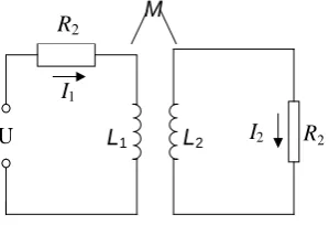Consequently, considering from the perspective of circuits, ECT is similar to the case of coupled inductance circuit, and the analysis of detecting coil impedance in eddy current testing can be discussed under the situation which is similar to two coupled coils [12].

An eddy current testing system can be equivalent to the equivalent circuit consisting of two inter-coupling coil, which is shown in Fig. 1. When an alternating current I1 passes through the primary side coil, the primary side coil is going to induce an alternating electromagnetic field, and the secondary side is going to induce a current to the effect of the electromagnetic field. At the same time, the induced current in a secondary side coils reacts upon the primary side through mutual inductance; in this case, the equivalent impedance can be used to express the effect on the primary side coil which is exerted by the secondary side coil.

Fig. 1: Mutual inductance circuit of coupled coils

At this moment, the impedance of coil 1 varies, the quantity of variation can be expressed with equivalent impedance (Zz=Rz+Xz) as below:

2 2

2 2

2 2 2 2

2 2 2 2

M M

z z

X X

R R X X

R X R X

= = −

+ + (2)

where X2=ωL2, XM =ωM.

The sum of equivalent impedance and primary side coil impedance is called apparent impedance (Z_s=R_s+X_s)

1

s z

R =R +R (3)

1

z z

X =X +X (4)

whereR1+X1=R1+j Lω 1 is apparent impedance of the primary side coil.

Knowing from the above definition of apparent impedance, the variation of apparent impedance to a circuit is going to draw the change of current or voltage in the primary side. As a result, the effect from the secondary side coil exerts on the primary side coil impedance can be back-stepped according to the impedance variation of the primary side circuit. Thereby, the impedance variation of the secondary side circuit can be calculated.

The value of two components Rs and Xs of apparent impedance by the primary side circuit can be achieved from

reducing the value of secondary side resistance R2 constantly from ∞ to zero, and draw the achieved value on a coordinate plane, which takes Rs as horizontal axis and ωL as a vertical axis, then a semicircle curve shown in

R1

L1 L2

I1

I2

M

R2 U

Figure 2 will be obtained, and the curve is called impedance plane diagram. The radius to the circle in Fig. 2 equals tok2

ω

2 2

1 2

/

k =M L L . Apparent reactance ωL monotone reduces from ωL1 to ωL1(1-K2), whereas apparent resistance R increases from R1 and after passing the maximum point (R1+k2ωL1/ 2), it decreases back to R1,

the parameter is R2 (

∞

∞

ωL1(1-K 2

)

ωL1

R2=∞/X2=0

A

Z0 Xs

Zm

B R2=0/X2=∞

R1 2 1 1

2 K L R+ ω Rs

Fig. 2: Impedance plane diagram of primary side coil when coils are coupled

(2) SKIN EFFECT

When alternating current energizes the exciting coil, the eddy current at certain depth induced in a test piece is going to generate a magnetic field whose direction is opposite to the original magnetic field and reduce the magnetic flux, then lead in the eddy current weaken in deeper layer. As a result, the density of eddy current becomes less with the distance to the surface increases. This variation depends on excitation frequency, the conductivity and the permeability of test piece, and the eddy current induced in a test piece concentrate at the surface of a test piece near the exciting coil. This phenomenon is called skin effect. Under the circumstances of the plane electromagnetic wave permeates into a semi-infinite conductor, the attenuation formula of eddy current shows below:

0 x f x

J =J e− π µσ (5)

In the formula, where J0 represents the density of eddy current on the surface of test piece, σ represents the conductivity of test piece, μ represents the permeability of a test piece, x represents the distance to the surface of test piece, Jx represents the density of eddy current lying in the test piece at the distance of x to the surface, f represents the frequency of exciting current. In order to indicate the depth of eddy current testing, usually define the depth where the density of eddy current reduces to 1/e times of it that is on a surface of a test piece as standard penetration depth (skin depth), expressed with δ. By equation (5):

1

f

δ

π µσ

= (6)

The formula is appropriate to the material of infinite thickness and the plane electromagnetic field. In the process of actual testing, the attenuation density quantity of eddy current is more than the value calculated by a skin depth formula. The difference of eddy current density indicates that the internal defects lying in different depth will change the probe impedance in varying degrees, and a big internal defect and a small external defect will generate signals of same amplitude. Therefore, it is not enough to estimate the severity of a defect only according to the change of signal’s amplitude, and make accurate judgment only if analyze the change of both signal’s amplitude and signal phase simultaneously.

EDDY CURRENT TESTING BASED ON FIELD ANALYSIS

______________________________________________________________________________

perturbed electromagnetic field around the Maxwell’s equations and their properties[13-15].

(1) TIME-HARMONIC ELECTROMAGNETIC FIELD MAXWELL’S EQUATIONS

When the field source varies sinusoidally in time, the stable-state electromagnetic field which is in linear medium and whose parameters do not change with time is a time-harmonic electromagnetic field. The electromagnetic field problems in eddy current testing can be simplified to analyze and solve the problems of time-harmonic electromagnetic field, besides, due to a non-sinusoidal periodic signal can be decomposed into a superposition of a series of sinusoidal signals, the solution of non-sinusoidal stable-state linear electromagnetic field can be obtained through solving the problems of time-harmonic field[16-17].

Take ejωt as a time-harmonic factor, ω>0, the Maxwell’s equations can be expressed into complex form in light of the corresponding relation between sinusoidal quantity and complex quantity:

( )

s

H J σ jωε E

∇× =  + +  ₍₇₎

E j Bω

∇× = −  ₍₈₎

0

B

∇ ⋅ = ₍₉₎

D ρ

∇ ⋅  =  (10)

In the formula, where H represents magnetic-field intensity, J_srepresents current density of external source,

Drepresents electric displacement, Brepresents magnetic induction intensity, Erepresents electric field intensity, ρrepresents free charge volume density. The complex form constraint equations significantly reduce the complexity of solving the solutions of field and remove the spot representing a complex number, likeBcan be written as B,

Ecan be written as E, etc.

(2) TIME-HARMONIC FIELD’S VECTOR MAGNETIC POTENTIAL AND ITS BOUNDARY VALUE PROBLEMS

In order to simplify the computing and analysis, we bring in vector magnetic potential A to describe the boundary value problems of time-harmonic field, so that the time-harmonic field Maxwell’s equations can be expressed with A

[18].

In vector analysis, it’s certain for any vector A:

( A) 0

∇ ⋅ ∇ × ≡ (11)

Contrast the equation (9) of time-harmonic field Maxwell’s equations, consider

B= ∇×A (12)

Plug equation (12) into equation (8) and get:

(E j Aω ) 0

∇ × + = (13)

In vector analysis, it’s constant for any scalar function φ

( j) 0

∇× ∇ ≡ (14)

Contrast equation (13) to (14), consider

E+ j Aω = −∇j, orE= −∇ −j j Aω (15)

here, φ represents scalar potential. According to equation (15) and (7), while use the relation equationB=

µ

( F) ( F) F

2

2 2

( )

s

k

A k A J A

j

µ j

ω

∇ + = − + ∇ ∇ ⋅ − (16)

where,_k2 _{= −j}ωµ σ_{( +j}ωε₎

.

On the other hand, use the relation equationD=εEand equation (15), the equation (10) can be written into

2j _jω _A ρ ε

∇ + ∇ ⋅ = − (17)

Equation (16) and (17) contain all the relation of Maxwell’s equations (7)-(10). For sake of solving equation (16) conveniently, it chooses the electromagnetic potential function (A, φ) which meets Lorentz gauge:

2

0

k A

jωj

∇ ⋅ − = (18)

Use Lorentz gauze, equation (16) and (17) respectively turn into:

2 2

s

A k A µJ

∇ + = − (19)

2 2

k ρ

j j

ε

∇ + = − (20)

After using Lorentz gauze, the inter-coupling of A and φ which present in origin equation (16) and (17) is separated. Vector magnetic potential A is known, and then could get the expression of scalar potential by using Lorentz gauze:

2

j A k

ω

j= ∇ ⋅ (21)

plug into equation (15), so the electric field intensity also can be expressed with vector magnetic potential:

2

1

[ ( )]

E j A j A A

k

ω j ω

= − − ∇ = − + ∇ ∇ ⋅ (22)

Equation (12) and (22) indicate that as long as determine a vector magnetic potential A uniquely, each component of electromagnetic is going to be ascertained uniquely.

(3) PERTURBEDMAGNETIC FIELD GENERATED BY IDEAL DEFECTS

So far, there have been massive research reports about the perturbed electromagnetic field caused by ideal defects. Typical eddy current testing problems can be described in Fig. 3: the exciting coil in air domain Va is the time-harmonic exciting source Js with factor ejωt, and a defect Vf is surrounded by conductor Vc. Usually makes the

exciting coil scan across the surface of test piece, and inspect defects through variations of scattered field. Assuming the interface between air and conductor is Sac, the interface between defect and conductor is Sdc, the conductivity of conductor domain is σc, the conductivity of defect domain is σf, and defect fulfills with air inside. The variation of electromagnetic field to the system caused by a defect is the key to field analysis [19-20].

Fig. 3: Typical eddy current testing problems

Define Ed and Bd as the difference between the field with defect and the field with no defect, which is:

d

k k ik

d

k k ik

B B B

E E E

 = −



 _{= −}



(23)

Vc(σ, μ0, ε0) Vd

Va(σ, μ0, ε0)

Js Sdc Sac

______________________________________________________________________________

where k＝a,c,f. We can get the equations as follows:

In air domain Va:

0

d a

B

∇× = (24)

d d

a a

E j Bω

∇× = − (25)

In conductor domain Vc:

0

d d

c c c

B µ σ E

∇× = (26)

d d

c c

E j Bω

∇× = − (27)

In defect domain Vf:

0 0

d

f f f c if B µ σ E µ σ E

∇× = − (28)

d d

f f

E j Bω

∇× = − (29)

If regard the (µ σ_{0 f}E_f −µ σ_{0 c}E_if ) in equation (28) as an equivalent current source, then the equations (24)-(29) have apparent physical meaning. It indicates the perturbed field can be regarded as being generated by equivalent current source of defect domain.

In the system described by Fig. 3, the vector magnetic potential in air generated by unit time-harmonic current dipole, which is in the conductor along x direction:

a ax az

A =A i+A k (30)

In there ' 0 0 2 ( )d 4 uz z ax j

A e J

u λ

λ _{λρ λ}

πω λ

∞ ₋

=

+

∫

' 1 0

2

cos ( )d

4

uz z az

j

A e J

u λ λ

j λρ λ

πω λ

∞ ₋

= −

+

∫

where r=(x, y, z) represents field point radius vector, ' ' ' '

( , , )

r = x y z represents source point radius vector,

'

R= −r r represents the distance field point and source point, ' 2 ' 2

(x x) (y y)

ρ= − + − ,

'

cosj=(x−x) /ρ,sinj=(y−y') /ρ, J0(⋅) and J1(⋅) represent zero order and first-order Bessel function respectively,

2 2

u= λ −k . Owing to the field, point lies in air domain and source point lies within a conductor domain, z>0,

'

0

z≤ .

Get the magnetic field B in air domain through vector magnetic potential A:

( x ) ( x)

z A z A

A A

B A i j k

y z x y

∂ ∂

∂ ∂

= ∇× = + − + −

∂ ∂ ∂ ∂ (33)

consequently ' 1 0 0 ( ) sin 2

[ - ( )]d

4

uz z x

J j

B e J

u

λ λρ

j λ _{λ λρ λ}

πω λ ρ

∞ ₋

=

+

∫

'

2

0 0

2

( )d cot

4

uz z

y x

j

B e J B

u

λ

λ _{λ λρ λ j}

πω λ

∞− ₋

= −

+

'

2

1 0

sin 2

( )d

4

uz z z

j

B e J

u

λ

j λ _{λρ λ}

πω λ

∞ ₋

=

+

∫

RELATIONS BETWEEN IMPEDANCE ANALYSIS AND FIELD ANALYSIS

In eddy current non-destructive testing, exciting coil generates induced eddy current through the conductor, and the distribution of eddy current influences the magnetic field surrounding exciting coil, which makes coil impedance engender an increment ΔZ. When there is defect existing in the conductor, the distribution of eddy current is disturbed and varies the increment of coil impedance. On the one hand, the ECT technology based on impedance analysis identifies the defect in light of the magnitude and phase of coil impedance increment ΔZ; On the other hand, the magnitude of perturbed magnetic field also reflects the situation of the defect. If detecting the size and distribution of the disturbed magnetic field, and through analyzing the perturbed magnetic field, it can also realize the identification of a defect, which is the ECT technology based on field analysis.

The relations between impedance analysis and field analysis can be converted through electromagnetic field equations, and the two analysis methods not only have close connection between, but also possess their respective advantages and disadvantages in detecting process [21]. For the solving region V, there are following relations between detecting probe impedance and electromagnetic field quantity seeking for solutions:

j

σ∗_{= +}σ ωε ₍₃₇₎

J∗ =σ∗E (38)

B E

t

∂ ∇× = −

∂ (39)

1 d 2 V

P J J V

σ

∗

=

_∫

2

P R

I

= (41)

where E represents magnetic-field intensity, B represents magnetic induction intensity, J represents the density of current, ε represents the dielectric constant, σ represents conductivity, I represents RMS value of current, P

represents the comic loss in a domain, V represents the electromagnetic field domain under solved. Using the above relations and it is possible to obtain the variation of probe impedance through the known electromagnetic field quantity in space and other electromagnetic parameters. Then connect the analysis methods based on impedance and on a field. The comparison of two methods is shown in Tab. 1.

According to the phase and amplitude of impedance increment, the ECT based on impedance analysis judges the existence of a defect in test piece and identifies the defect. Generally speaking, the response of detecting coil reaches the maximum when the coil is responding to its surrounded area and to the material able to change total magnetic flux through the coil. As a result, when find out the defect with larger size, applying coil detect and impedance analysis has more advantages. The distribution of perturbed magnetic field cannot be interpreted due to the coil impedance variation ΔZ is just integration effect of perturbed magnetic field in detecting coil volume. When detecting the defect in multilayer conductive structure, in order to achieve greater penetration depth the excitation frequency has to be decreased, and this will reduce the amplitude of induced voltage, which means the sensitivity of a probe reduces with excitation frequency decreases. In order to solve this problem, it’s good to use high-powered exciting coil, to increase the turns of coil and to enlarge the radius of the probe; but this will make the exciting coil impossible to have small size, while the inspection will not be able to obtain a high space resolution and to detect the small-size defect in deep layer.

______________________________________________________________________________

low frequency; the sensors can be made quite small at the same time, and the detecting signal distortion is also very little, so it’s able to detect the small-size defect in deep layer.

Tab. 1: Comparison of impedance analysis and field analysis

Detection method

ECT based on field analysis

ECT based on impedance analysis Detection

object space magnetic field B coil impedance increment ΔZ

Probe layout

exciting probe and detecting probe are separated, exciting probe use coil sensor, detecting probe use magnetic field sensor, very small size, able to constitute an array

exciting coil and detecting coil can be separated or be united as one, exciting probe and detecting probe both use coil sensor, relatively larger size

Probe detection

situation relatively high scan speed relatively low scan speed Spatial

resolution

spatial resolution equals to scale of magnetic field sensor, subtle, able to detect small-size defect

spatial resolution equals to scale of coil, unsubtle, unable detect small-size defect

Defect identification

analyze the distribution of space magnetic field, good performance at low frequency, greater penetration depth, identify defect in deep layer

analyze the impedance plane diagram, low sensitivity at low frequency, only able to detect the defect on surface and near surface

Direct problem

solve the distribution of space magnetic field from source (exciting source, defect), only need to solve eddy current field problems once in each time of analysis

solve the distribution of space magnetic field from source (exciting source, defect) and then solve coil impedance, need to solve eddy current field problems many times in each time of analysis to get impedance curve

Inverse problem

solve the source from the distribution of space magnetic field, the corresponding relation is relatively direct

solve the source from coil impedance variation, the corresponding relation is not direct

CONCLUSION

This paper mainly researches on the theoretical basis of eddy current testing, and lays stress on discussing the two common analysis methods in ECT: impedance analysis method and field analysis method, then analyzes and contrasts the two methods in depth, while puts forward the inner connection of two methods and their respective characteristics. Due to the difference of detecting device, the ECT based on field analysis has higher sensitivity, spatial resolution and speed in detection than the ECT based on impedance analysis.

Acknowledgments

This work is supported by the National Natural Science Foundation of China Grant No. 51105183, 51307172, the Research Fund for the Doctoral Program of Higher Education of China Grant No. 20115314120003, the Applied Basic Research Programs of Science and Technology Commission Foundation of Yunnan Province of China Grant No. 2010ZC050, the Foundation of Yunnan Educational Committee Grant No. 2013Z121, the National College Student Innovation Training Program Funded Projects Grant No. 201210674014, the Science and Technology Project of Yunnan Power Grid Corporation Grant No. K-YN2013-110.

REFERENCES

[1]H Fukutomi; T Takagi; M Nishikawa, NDT & E Int., 2001, 34(1), 17–23.

[2]N Yusa; L Janousek; M Rebican; Z Chen; K Miya; N Chigusa; H Ito, Nucl. Eng. Des., 2006, 236(18), 1852–1859.

[3]Z Riadh; D Bernard; L Dominique; P Francis, IEEE Trans. Magn., 1991, 27(6), 4416-4437. [4]K Schmidt; O Sterz; R Hiptmair, IEEE Trans. Magn., 2008, 44(6), 686-689.

[5]AL Kholmetskii; OV Missevitch; T Yarman, Eur. J. Phys., 2008, 29 (3) N5-N10. [6]K Miya, IEEE Trans. Magn., 2002, 38(2), 321-326.

[7]JR Bowler, Int. J. Appl. Electrom., 1997, 8, 3-16.

[8]S Ananth; R James, J. Nondestruct. Eval., 1995, 14(1), 39-46. [9]A Kameari, IEEE Trans. Magn., 1988, 24, 118-121.

[10]K Ishibashi, IEEE Trans. Magn., 1995, 31(3), 1500–1503. [11]S Norton; J Bowler, J. Appl. Phys., 1993, 73, 501-512. [12]K Ishibashi, IEEE Trans. Magn., 1994, 30(5), 3020–3023.

[13]VV Dyakin; VA Sandovskii; MS Dudarev, Russ. J. Nondestruct. Test., 2004, 40(8), 533-540. [14]Z Zeng; L Udpa; SS Udpa; M Shiu; C Chan, IEEE Trans. Magn., 2009, 45(3), 964-966. [15]K Ishibashi, IEEE Trans. Magn., 2001, 37(5), 3229-3231.

[16]JH Bramble; TV Kolev; JE Pasciak, J. Numer. Math., 2005, 13(4), 237-263.

[18]D Patrick; G Johan; G Christophe; S Nelson; J Bastos, IEEE Trans. Magn., 2003, 39(3), 1424-1427. [19]Z Chen; K Aoto; K Miya, IEEE Trans. Magn., 2000, 36(4), 1018-1022.