Multivariate quality control using an integrated artificial neural network scheme: a case study in plastic injection molding industry

MULTIVARIATE QUALITY CONTROL USING AN INTEGRATED

ARTIFICIAL NEURAL NETWORK SCHEME: A CASE STUDY IN

PLASTIC INJECTION MOLDING INDUSTRY

AFIZ AZRY MOHD KHAIRY

Tesis ini dikemukakan sebagai memenuhi syarat penganugerahan

Ijazah Sarjana

Fakulti Kejuruteraan Mekanikal dan Pembuatan Universiti Tun Hussein Onn Malaysia

ABSTRACT

ABSTRAK

TABLE OF CONTENTS

MULTIVARIATE QUALITY CONTROL USING AN

INTEGRATED ARTIFICIAL NEURAL NETWORK SCHEME: A CASE STUDY IN PLASTIC INJECTION MOLDING

INDUSTRY ... iii

ACKNOWLEDGEMENT ... iii

ABSTRACT ... iv

ABSTRAK ... v

TABLE OF CONTENTS ... vi

LIST OF TABLE ... ix

LIST OF FIGURE ... xi

LIST OF SYMBOL ... xiii

LIST OF APPENDIX ... xiv

CHAPTER 1 ... 1

INTRODUCTION ... 1

1.1 Project Background ... 1

1.2 Problem Statements ... 2

1.3 Project Objectives ... 3

1.4 Project Scopes ... 3

1.5 Dissertation Outline ... 3

CHAPTER 2 ... 5

LITERATURE REVIEW... 5

2.1 Statistical process control (SPC) ... 5

2.2 Univariate Control Chart ... 7

2.2.1 Shewhart Control Chart... 8

2.2.3 Average Run Length (ARL)... 9

2.2.4 Patterns of Process Behavior ... 10

2.2.5 Control Chart for Mean - Chart ... 11

2.2.6 Control Chart for Process Variation R- Chart ... 12

2.2.7 Individuals Control Charts ... 13

2.3 Exponential Weighted Moving Average (EWMA) Chart ... 14

2.4 Multivariate Control Chart ... 15

2.4.1 Hotelling’s T2 Chart ... 16

2.4.2 MEWMA Control Chart ... 20

2.4 Advances statistical process control ... 20

2.4.1 ANN-based model: Novelty Detector-ANN ... 21

2.4.2 ANN-based model: Modular-ANN scheme ... 22

2.4.3 ANN-based model: Ensemble-ANN ... 22

2.4.4 ANN-based model: Multi modules-ANN scheme ... 24

2.4.5 Integrated MSPC-ANN ... 24

2.4.6 Monitoring and diagnosis of Bivariate process mean shitfts’ schemes ... 26

2.5 Artificial Neural Networks (ANN) ... 33

2.6 Previous study ... 35

CHAPTER 3 ... 39

METHODOLOGY ... 39

3.1 Introduction ... 39

3.2 Bivariate Mean Shift ... 39

3.3 Problem Situation and Solution Concept ... 41

3.3.1 Case Study in industry ... 41

3.4 Project Methodology ... 42

3.5 Selection type of specimen... 43

3.6 Experiment Work ... 43

3.6.1 Experiment procedure steps ... 45

3.7 Control Chart ... 46

3.8 Result Analysis ... 46

3.8.1 Selection of bivariate dependent variables. ... 47

3.8.3 Data Pattern interpretation ... 47

3.8.4 Performance comparison ... 48

CHAPTER 4 ... 49

RESULTS AND DISCUSSIONS ... 49

4.1 Introduction ... 49

4.2 Result validation ... 49

4.3 Industrial result... 49

4.4 Variables selection ... 49

4.5 Univariate Control Chart interpretation ... 50

4.6 Multivariate SPC chart result ... 52

4.7 Advance SPC Chart ... 53

4.8 Out of control recognition performance comparison ... 53

4.8.1 I-Chart for performance reference ... 57

4.8.2 T2 Chart for performance reference ... 58

4.8.3 MEWMA-ANN scheme detection performance ... 59

4.8.4 Statistical Features scheme detection performance... 60

4.8.5 Baseline scheme detection performance ... 61

4.8.6 Summary of rapid recognition performance ... 62

4.8.7 Advances SPC Scheme diagnosis accuracy ... 63

4.9 Results Summary ... 67

CHAPTER 5 ... 68

CONCLUSIONS AND RECOMMENDATIONS ... 68

5.1 Introduction ... 68

5.2 Conclusions ... 68

5.3 Project Contribution ... 69

5.4 Future Work Recommendations ... 70

5.5 Closing Note ... 70

REFERENCES ... 71

APPENDIX ... 75

LIST OF TABLE

3.1 Part information... 43

3.2 Tooling information ... 43

3.3 Process variables in Plastic Injection ... 44

4.1 Recognition performance between I-Chart and EWMA Chart ... 50

4. 2 Correlation Coefficient from various combinations. ... 54

4. 3 MEWMA-ANN scheme for 20% Regrind resin mixed for Variable A and C from cavity no.1 ... 59

4.4 MEWMA-ANN scheme for Injection Speed Up 5% for Variable A and C from cavity no.2 ... 60

4.5 MEWMA-ANN scheme for Holding Pressure Up 5% for Variable B and C from cavity no.1 ... 60

4.6 Statistical Features scheme for 20% Regrind resin mixed for Variable A and C from cavity no.1 ... 60

4.7 Statistical Features scheme for Injection Speed Up 5% for Variable A and C from cavity no.2 ... 61

4.8 Statistical Features scheme Holding Pressure Up 5% for Variable B and C from cavity no.1 ... 61

4.9 Baseline scheme for 20% Regrind resin mixed for Variable A and C from cavity no.1 ... 61

4.10 Baseline scheme for Injection Speed Up 5% for Variable A and C from cavity no.2 ... 62

4. 11 Baseline scheme Holding Pressure Up 5% for Variable B and C from cavity no.1 ... 62

4.12 MEWMA-ANN scheme ... 62

4.13 Statistical Features scheme ... 63

4.15 Diagnosis accuracy for Variable A and C in 20% Regrind resin mixed from cavity no.1 - correlation

coefficient 0.187 ... 64 4.16 Diagnosis accuracy for Variable A and C Injection

Speed Up 5% from cavity no.2 - correlation coefficient

0.476 ... 64 4.17 Diagnosis accuracy for Variable B and C in Holding

Pressure Up 5% from cavity no.1 - correlation

coefficient 0.901 ... 64 4.18 Diagnose performance of MEWMA-ANN scheme for

Mean shifts condition and total process ... 65 4.19 Diagnose performance of Statistical Features scheme

for Mean shifts condition and total process ... 65 4. 20 Diagnose performance of Baseline scheme for Mean

shifts condition and total process ... 65 4. 21 Magnitude value of Mean Shifts from In Control

LIST OF FIGURE

2.1 Cp condition for varying process widths ... 7

2.2 How the Control Chart works ... 9

2.3 Trend of sudden shifts patterns ... 10

2.4 The Western Electric run rules. ... 11

2.5 -Chart (above) and R-Chart (below) ... 13

2.6 Individual Chart shows the process is in control, since none of the plotted points fall outside either the UCL or LCL. ... 14

2.7 EWMA Chart ... 15

2.8 A generic bivariate Hotelling’s T2 control region ... 17

2.9 A generic T2 control chart ... 19

2.10 Advances in SPCPR schemes ... 21

2.11 Novelty detector-ANN recognizer (Zorriassatine et al., 2003)... 22

2.12 Modular-ANN scheme (Guh,2007) ... 23

2.13 Ensemble-ANN recognizer (Yu and Xi, 2009) ... 24

2.14 Multi-modules-ANN scheme (El-Midany et al., 2010) ... 25

2.15 he integrated MSPC-ANN schemes ... 26

2.16 Framework for the Baseline scheme ... 27

2.17 Framework for the Statistical Features ANN scheme ... 29

2.18 Framework for the Synergistic-ANN scheme schemes ... 30

2.19 Framework for MEWMA-ANN schemes ... 32

2.20 Structure of a back propagation network (BPN) ... 34

2.21 Structure of a learning vector quantization (LVQ) networks ... 34

3.2 Overview of Project Methodology ... 42 3.3 Effect of variation in material regrind levels ... 44 3.4 Monitoring Process Variables versus Monitoring

Process Output... 44 4.1 I –Chart for A,B & C ... 51 4.2 EWMA Chart for Variables from Cavity 1 and Cavity 2

in various process continues changed from Holding Pressure ,Injection Speed, mixed 20% and 50% regrind

resin ... 51 4.3 a) T2 chart, b) MEWMA chart ... 52 4.4 Scatter Plot for variables at Holding Pressure

disturbance ... 55 4.5 Scatter Plot for variables at Injection Speed disturbance ... 56 4.6 Scatter Plot for variables at use of Regrind resin

disturbance ... 56 4.7 I-Chart for 20% Regrind resin mixed for Variable A

and C from cavity no.1 ... 57 4.8 I-Chart for Injection Speed Up 5% for Variable A and

C from cavity no.2 ... 57 4.9 I-Chart for Holding Pressure Up 5% for Variable A and

C from cavity no.1 ... 58 4.10 T2 Chart for variables’ combinations from low ~ high

LIST OF SYMBOL

α - Type I error (α risk)

β - Type II error (β risk)

λ - Constant parameter for EWMA control chart

ρ - Correlation coefficient for bivariate samples

μ - Mean

σ - Standard deviation

μ

0 - Mean for in-control samples

σ

0 - Standard deviation for in-control samples

σ

ij - Covariance for bivariate samples

Σ - Covariance matrix for bivariate samples or basic summation X

t - Original observation samples at time/point t Z

t - Standardized observation samples at time/point t N - Random normal variates

- Sample mean

X2 - Hotelling’s generalized distance

S - Hotelling’s covariance of sample

LIST OF APPENDIX

Appendix A: Factors Used When Constructing Control Charts ... 75 Appendix B: Various process continues changed from In Control

Process used 100% virgin resin till mixed with 50%

regrind resin. ... 76 Appendix C: In Control Process changed to Holding Pressure 5%

decreased ... 78 Appendix D: In Control Process changed to Holding Pressure 5%

increased ... 80 Appendix E: In Control Process changed to Injection Speed 5%

increased ... 81 Appendix F: In Control Process changed to Injection Speed 5%

decreased ... 82 Appendix G: In Control Process changed to mixed with 20%

Regrind resin ... 83 Appendix H: In Control Process changed to mixed with 50%

CHAPTER 1

INTRODUCTION

1.1 Project Background

1.2 Problem Statements

To produce product that meet the specification requirement is the important point that lead them to control and monitor the quality in the process. In manufacturing process, quality monitoring is practice by sampling check on the bulk lots which produced at specific interval of in control process running time according to standard specification. Easy to implement, less investment and applicable to any kind of environment are the reasons why traditional SPC method is common in most of the manufacturing industries. The control charts in traditional SPC are designed to monitor a single product with large production runs. But imbalance in monitoring and diagnosis of multivariate process variation, most of the problems cannot be detected in advance that lead to poor Quality control in manufacturing , rework, scrap, product failures and recalls can severely damage the company business. In addition, process variation from 4Ms (Man, Machine, Material, and Method) contribute to the process quality. The research activity in multivariate control charts has been reported to be at its highest level for the past decade which reflects increased measurement and computing ability (Woodall & Montgomery, 1999). Large and diversified research areas on the application of multivariate control charts in manufacturing areas are extensively discussed in many literatures (Tracy, Mason and young (1992), Lowry and Montgomery (1995), Mason and young (2002) and the references therein).

1.3 Project Objectives

The objectives of this project are:

i. To investigate the effectiveness of the Integrated MEWMA-ANN scheme in monitoring and diagnosing process faults in manufacturing industry

ii. To recognize problems or drawbacks arise from Integrated MEWMA-ANN scheme and discuss the proposal for improvement of scheme.

1.4 Project Scopes

The scopes of this project are:

i. The application of Univariate Statistical Process Control Chart which are Individual Chart and Exponentially Weighted Moving Average (EWMA) Charts

ii. The application of Multivariate Statistical Process Control Chart which are Hotelling T Square Chart and Multivariate Exponentially Weighted Moving Average (EWMA) Charts

iii. The application of Advance Statistical Process Control chart which are Baseline artificial neural network (ANN) pattern recognitions scheme, Statistical Features artificial neural network (ANN) pattern recognitions scheme and Integrated MEWMA-ANN artificial neural network (ANN) pattern recognition scheme

iv. Thermo plastic part fabricated from Plastic Injection Process machine which the dimensions and weight were differed base on the changes in machine parameter and the usage of virgin plastic resin mixed with 20% and 50% of regrind plastic resin.

1.5 Dissertation Outline

This dissertation is organized as follows: Chapter I

Chapter II

This chapter is a review of SPC fundamental knowledge describing on the function and application of each type control chart by previous researcher and practitioner. Chapter III

This chapter elaborates the methodology used in this project. Chapter IV

This chapter presents the result of performance of recognizing process out of control by Univariate SPC, Multivariate SPC and Advance Multivariate SPC. The diagnosing accuracy of MEWMA-ANN scheme, Statistical Features scheme and Baseline scheme were compared.

Chapter V

CHAPTER 2

LITERATURE REVIEW

2.1 Statistical process control (SPC)

Variation in manufacturing process environment causes no parts or products can be produced in exactly the same size and properties. Process variation can be influenced from chance causes (random error) and/or assignable causes (systematic errors) (Montgomery, 2009). There are many ways to implement process control. Key monitoring and investigating tools include:

i. Histograms ii. Check Sheets iii. Pareto Charts

iv. Cause and Effect Diagrams v. Defect Concentration Diagrams vi. Scatter Diagrams

vii.Control Charts

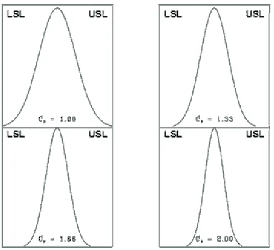
The underlying concept of statistical process control is based on a comparison of what is happening today with what happened previously. Stated differently, we use historical data to compute the initial control limits. Then the data are compared against these initial limits. Points that fall outside of the limits are investigated and, perhaps, some will later be discarded. Process capability compares the output of an in-control process to the specification limits by using capability indices. The comparison is made by forming the ratio of the spread between the process specifications (the specification "width") to the spread of the process values, as measured by 6 process standard deviation units (the process width").The definition of the Cp given in Equation (2.1) implicitly assumes that the process is centered at the nominal dimension.

s

6 LSL USL

C_p = - (2.1)

If the process is running of center, it actual capability will be less than indicated by the Cp. It is convenient to think of Cp as a measure of potential capability, that is, capability with centered process. If process is not centered, a measure of actual capability is often used. This ratio is called Cpk as defined in Equation (2.2).

úû ù êë

é -

-=

s m s

m 3 , 3

min USL LSL

Cpk (2.2)

Figure 2.1: Cp condition for varying process widths

The aim of statistical process control (SPC) is to achieve higher quality of final product and lower the production loss due to defect product. Process monitoring with control chart is a basic tool of statistical process control. It monitors the behavior of a production process and signals the operator to take necessary action when abnormal event occurs. A stable production process is the key element of quality improvement. Depending on the number of process characteristics to be monitored, there are two basic types of control charts, Univariate Control Chart and Multivariate Control Chart .

2.2 Univariate Control Chart

monitor such variables separately using univariate SPC charting scheme would increase false alarms and leading to wrong decision making. However, monitoring each process variable with separate Shewhart control chart ignores the correlation between variables and does not fully reflect the real process situation. Nowadays, the process industry has become more complex than it was in the past and inevitably that number of process variables need to be monitored has increased dramatically. Thus only monitor a single parameter or output at a time. Therefore they cannot detect changes in the relationship between multiple parameters. Very often, these variables are multivariate in nature and using Shewhart control charts becomes insufficient.

2.2.1 Shewhart Control Chart

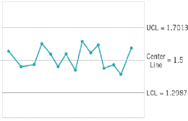
The most common use method in current industries is Control Chart or Shewhart

Charts. These control charts are constructed by plotting product’s quality variable

over time in sequence plot as shown in Figure 2.2. A control chart contains a center

line, an upper control limit and a lower control limit. Points that plots within the

control limits indicates the process is in control. In this condition no action is necessary. Points that plots outside the control limits is evidence that the process is out of control. In this condition, investigation and corrective action are required to find and eliminate assignable cause(s) (Mendenhall & Sincich, 2007).

Let w be a sample statistic that measure some quality characteristic of interest and suppose that the mean of w is µw and the standard deviation of w is σw. Then the center line, upper control limit and lower control limit as shows in equation (2.3).

UCL = µW+ LσW

Center Line = µW (2.3)

LCL = µW - LσW

Where L is “the distance” of the control limits from center line, expressed in standard

Figure 2.2: How the Control Chart works

2.2.2 Control Limits

A point falling within the control limits means it fails to reject the null hypothesis that the process is statistically in-control, and a point falling outside the control limits means it rejects the null hypothesis that the process is statistically in-control.

Therefore, the statistical Type I error α (Rejecting the null hypothesis H0 when it is true) applied in Shewhart control chart means the process is concluded as out-of-control when it is truly in-control. Same analog, the statistical Type II error β

(Failing to reject the null hypothesis when it is false) means the process is concluded as in-control when it is truly false.

2.2.3 Average Run Length (ARL)

The performance of control charts can also be characterized by their average run length. Average run length is the average number of points that must be plotted before a point indicates an out-of-control condition (Montgomery, 1985). We can calculate the average run length for any Shewhart control chart according to,

p

Where p or Type I error is the probability that an out-of-control event occurs. Therefore, a control chart with 3 sigma control limits, the average run length will be

370 0027 . 0

1 1

= =

=

p ARL

This means that if the process remains in-control, in average, there will be one false alarm every 370 samples.

2.2.4 Patterns of Process Behavior

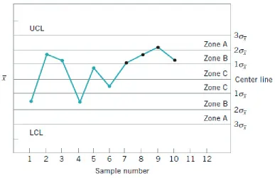
Apart from all the measurement should fall with the control limits, the process can be viewed as in-control when there is no systematic pattern shown in the process behavior. Systematic patterns occurring in Shewhart control charts have often been interpreted as indicators of extraneous sources of process variation (Mason, et al. 2003). The process will be improved if the causes of systematic pattern in the process are diagnosed and further eliminated. A statistically in-control process can be indicated by normal pattern, whereas out-of-control process can be indicated by abnormal patterns (upward shift, downward shift, upward trend, downward trend, cyclic, systematic, stratification, and mixture). Figure 2.3 shows in practice, sudden shifts patterns (upward or downward shift) commonly indicate there are changes in material, operator or machine. Trends patterns (upward or downward trend) indicate there are wears and tears in cutting tools. Cyclic patterns indicate there are voltage fluctuations in power supply (Chen et al., 2007).

The Western Electric Handbook (1956) provides a set of guidelines to detect the systematic patterns in the process. A brief summary is shown below. A process is considered as out-of-control if any of the following conditions holds:

i. One point falls outside the 3-sigma control limits (beyond Zone A).

ii. At least two out of three consecutive points fall on the same side of the centerline, and are beyond the 2-sigma control limits (in Zone A or beyond). iii. At least four out of five consecutive points fall on the same side of the center

line and are beyond the 1-sigma limits (in Zone B or beyond).

iv. At least eight successive points fall on the same side of the center line.

Figure 2.4:The Western Electric run rules.

2.2.5 Control Chart for Mean - Chart

R A x UCL R A x UCL x x Line Center k i i 2 2 1 -= + = =

=

å

(2.5)

Where

k = Number of samples, each of size lot i = Sample mean for the ith sample Ri = Range of ith sample

k R R k i i

å

A2 is given in table of Appendix B

2.2.6 Control Chart for Process Variation R- Chart

In Quality Control variability value of some quality characteristic can be controlled.

An increase in the process standard deviation σ means that the quality characteristic

variable will vary over a wider range, thereby increasing the probability of producing an inferior product (Mendenhall & Sincich, 2007). The variation in quality characteristic is monitor using a range chart or R-chart. The location of Center Line and Control Limits for R-chart are mentioned in equation (2.6)

R D UCL R D UCL R line Center 3 4 = = = (2.6) Where

k = Number of samples, each of size lot Ri = Range of ith sample

k R R k i i

å

and D3 and D4 are given in Table in Appendix B for n =2 to n =25

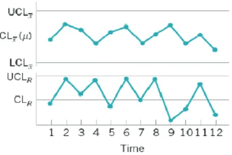
Figure 2.5: -Chart (above) and R-Chart (below)

2.2.7 Individuals Control Charts

The individuals control chart examines variation in individual sample results over time as shown in Figure 2.6. While rational subgrouping does not apply, thought must be given to when the results will be measured. If the process is in statistical control, the average on the individuals chart is our estimate of the population average. The average range will be used to estimate the population standard deviation. For individual measurements, e.g., the sample size = 1, use the moving range of two successive observations to measure the process variability. The moving range is defined as in equation (2.7)

1

-= _{i i}

i x x

MR (2.7)

Which is the absolute value of the first difference (e.g., the difference between two consecutive data points) of the data. Analogous to the Shewhart control chart, one can plot both the data (which are the individuals) and the moving range. For the control chart for individual measurements, the lines plotted are:

128 . 1 3

128 . 1 3

MR x

LCL

x Line Center

MR x

UCL

-=

= + =

Where is the average of all the individuals and is the average of all the moving ranges of two observations. Keep in mind that either or both averages may be replaced by a standard or target, if available. (Note that 1.128 is the value of d2 for n = 2) in Appendix B.

Figure 2.6: Individual Chart shows the process is in control, since none of the

plotted points fall outside either the UCL or LCL.

2.3 Exponential Weighted Moving Average (EWMA) Chart

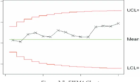
The Exponentially Weighted Moving Average (EWMA) control chart (Figure 2.7) is one of the control charts used to detect the occurrence of a shift in a process mean compared to widely used Shewhart control chart (Montgomery, 2009). The EWMA is used extensively in time series modelling and in forecasting.Upper Control Limit (UCL), Control Limit (CL) and Lower Control Limit (LCL) for the EWMA control chart are given below in the equation form respectively. According to Sharaf El-Din (2006) in [ Statistical Process Control Charts Applied to Steelmaking Quality Improvement ] values of λ in the interval 0.05 ≤ λ ≤ 0.25 work well in practice, with λ = 0.05, λ = 0.10, and λ = 0.20 being popular choices. A good rule of thumb is to use smaller values of λ to detect smaller shifts. The width of control limits L = 3 (the usual 3-sigma limits) works reasonably well, particularly with the larger value of λ, although when λ is small, say λ ≤ 0.10, there is an advantage in reducing the width of

[

]

λ = 0.1

σ = standard deviation of the object xi L = width of the control limits

Zi = Weighted average of all previous sample means.

Figure 2.7: EWMA Chart

2.4 Multivariate Control Chart

It is a graphical display of a statistic that summarizes or represents more than one quality characteristic. In the related study, many manufacturing processes involve two or more dependent variables, whereby an appropriate scheme is required to monitor and diagnose such variables jointly. This joint monitoring-diagnosis concept is called multivariate quality control (MQC). The T

2

control chart (Hotelling, 1947) that is developed based on logical extension of univariate SPC chart (Shewhart control chart) was claimed as an original work in MSPC. Nevertheless, it was found

deviations). In order to improve capability for detecting mean shift in smaller magnitudes (< 1.5 standard deviations), the multivariate cumulative sum (MCUSUM) (Crosier, 1988; Pignatiello and Runger, 1990) and the multivariate exponentially weighted moving average (MEWMA) (Lowry et al., 1992; Prabhu and Runger, 1997) control charts were developed based on logical extension of univariate CUSUM and EWMA control charts respectively. These multivariate control charts are commonly known as the traditional MSPC charting schemes. Aparisi and Haro (2001) proposed the T

2

control chart for variable sampling interval (VSI) to improve sensitivity in detecting mean shifts. Khoo and Quah (2003) developed a multivariate control chart for monitoring shifts in the covariance matrix based on individual observations. Alwan and Alwan (1994), Apley and Tsung (2002), and Jiang (2004) investigated the application of T

2

control chart for monitoring mean shifts in univariate autocorrelated processes. Ngai and Zhang (2001) proposed the MCUSUM control chart based on projection pursuit to deal with a specific situation, that is, the process mean is already shifted at the time the control charting begins. The traditional MSPC charting schemes are only effective for monitoring (detecting) mean shifts but they are unable to diagnose (identify) the sources of variation in mean shifts. In other word, it is unable to provide diagnosis information for a quality practitioner towards finding the root cause errors and solution for corrective action. Basically, the MSPC charting schemes for variables can be categorized to: (i) statistical design, and (ii) economical design. Both design categories can be further classified to fixed sampling interval (FSI) and variable sampling interval (VSI). The traditional MSPC charting schemes that are T

2

, MCUSUM and MEWMA control charts were designed based on statistical consideration for dealing with FSI.

2.4.1 Hotelling’s T2 Chart

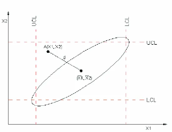
Hotelling H. (1931) can be viewed as the originator of multivariate control charts. Hotelling proposed a concept of generalized distance between a new observation to its sample mean. In case of bivariate condition by assuming these x1 and x2 are distributed according the bivariate normal distribution. Referring to Figure 2.8, say

Figure 2.8: A generic bivariate Hotelling’s T2 control region

The covariance s12 is used to estimate the dependency between x1 and x2. The generalized distance between point A and its mean can be calculated as:

[

]

1 1 22 1 1 2 2 2 2 2 11 2 22 22 11 2

0 ( ) 2( )( ) ( )

1 x x s x x x x x x s s s s

X - - - - +

-= (2.10)

This statistic follows the Chi-square distribution with two degrees of freedom. An ellipse can be graphed with the x1 and x2 in this equation. Moreover, all the points lying on the ellipse will generate the same Chi-square statistic. As a consequence, every observation can be determined whether its generalized distance exceeds the ellipse by comparing X02 and X22,α ,where X22,αis the upper α percentage point of the

Chi-square distribution with 2 degrees of freedom. The observation will be considered as out-of-control if X02 > X22,α

With the same concept of the generalized distance, it can be extended from bivariate to a multiple p variables. Let Xi =(Xi1,Xi2,….Xip) represent a p dimensional vector of measurements made on a process time period i. The value Xij represents an observation on the jth characteristic. Assuming that when the process is in control, the Xi are independent and follow a multivariate normal distribution with mean vector μ

Phase I and Phase II

The application of Hotelling’s T2 statistic shall be categorized into two phases. Phase I tests whether the preliminary process was in control and phase II tests whether the future observation remains in-control (Alt, 1985). Phase I operation refers to the construction of in-control data set. Same idea as Shewhart control chart, control limits are estimated from a period of in-control data.

To obtain this in-control data, the raw data set needs to be purged. For instance, the outliers need same idea as Shewhart control chart, control limits are estimated from a period of in-control data. To obtain this in-control data, the raw data set needs to be purged. For instance, the outliers need to be removed and the missing data needs to be substituted with an estimate. During phase I operation, Hotelling’s T2 statistic is calculated for each measurement and compared to the control limit, which will follows Chi-square distribution (according to Richard, A.J. & Dean, W.W., 2002.)

) ( ~ ) ( )

( 1 2_,

2 on distributi square Chi X X X S X X

T = _i - - _i - _ap - (2.11)

Also other research shows that the control limit follows Beta distribution (Mason, Young & Tracy,1992).

) 2 1 , 2 , ( 2 1

2 _{( ) ( )~} ( 1)

-- _-

-= _{i i} B _{pn p}

n n X X S X X T

a (2.12)

n=number of preliminary observations

Both control limits will be approximate when the number of observations is large. The control limit based on Chi-square distribution is established on the assumption that X and S are true values μ and Σ, which is just an approximate

situation (Mason, Young & Tracy, 1992). Beta distribution is more precise and is a

) , , ( 1 2 ) ( ) 1 )( 1 ( ~ ) ( )

( _{i i} F_{pn pa}

p n n n n p X X S X X

T -

-+ -= (2.13)

Where sample mean is and the covariance of sample

pp p p S S S S S S S S s . . 2 23 22 1 13 12 11 =

The idea of using Hotelling’s T2 statistic in phase I and phase II is the same. Each measurement is examined whether it is out-of-control by checking if it deviates extraordinarily from its sample mean. It should be reminded to choose the correct upper control limit on different purposes.

The Hotelling’s T2 statistic can be extended for more than two variables. Instead of a 2-dimensional ellipse control region, the result will be presented in a similar way as Shewhart control chart. The T2 statistics calculated from all the observation will be plotted in a chart against time or observation serious and compared to the upper control limit. Figure 2.9 is a generic T2 control chart. It should be noticed that there is no center line and the lower control limit is set to zero, because the meaning of T2 statistic is a generalized distance between the observation and its sample mean.

2.4.2 MEWMA Control Chart

The MEWMA control chart is very sensitive in detecting small shifts (≤ 1.00

standard deviations) as compared to the T2 control chart. The MEWMA control chart developed by Lowry et al (1992) is a logical extension of the univariate EWMA control chart. In the bivariate case, the MEWMA statistics can be defined as follows:

MEWMAi = [σ22(EWMA1i –μ1)2+ σ12(EWMA2i–μ2)2

–2σ122(EWMA1i–μ1)(EWMA2i–μ2)] n / (σ12σ22–σ122 ) (2.14)

EWMA1i= λ Z1i + (1 –λ) EWMA1i-1 (2.15)

EWMA2i= λ Z2i + (1 –λ) EWMA2i-1 (2.16)

Covariance matrix of MEWMA:

ΣMEWMA = (λ / (1 –λ)) [ (σ12σ12) (σ12σ22) ] (2.17)

The σ1 = σ2 = 1; σ12= ρ. Notations λ and i represent the constant parameter and the number of samples. The starting value of EWMA (EWMA0) was set as zero to

represent the process target (μ0).

The MEWMA statistic samples will be out-of-control if it exceeded the control limit (H). In this study design parameter H=8.64 was used.

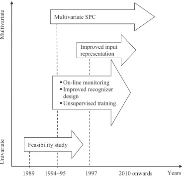
2.4 Advances statistical process control

Novelty Detector-ANN, Modular-ANN, Ensemble-ANN, Multi Modules-ANN scheme etc have been designed to perform process monitoring and diagnosis simultaneously and continuously.

Figure 2.10: Advances in SPCPR schemes

2.4.1 ANN-based model: Novelty Detector-ANN

Zorriassatine et al. (2003) applied single ANN recognizer, namely, novelty detector-ANN as shown in Figure 2.11 for recognizing normal pattern and sudden shift patterns (upward shift and downward shift).This scheme was effective to accurately identify the existence of mean shifts when dealing with large magnitudes of mean

shifts (≥ 2.0 standard deviations). However, there is difficult to identify the source of

variation when involving small magnitudes of mean shifts (1.0 standard deviation).

Univa

ria

te

Mul

ti

va

ria

te

1989 1994~95 1997 2010 onwards Years

Improved input representation Multivariate SPC

§On-line monitoring

§Improved recognizer design

§Unsupervised training

Figure 2.11: Novelty detector-ANN recognizer (Zorriassatine et al., 2003)

2.4.2 ANN-based model: Modular-ANN scheme

Guh (2007) proposed the modular ANN scheme as shown in Figure 2.12 for monitoring and diagnosis of bivariate process mean shifts. The study focused on the overall monitoring-diagnosis performances. In monitoring aspect, this scheme can be observed as so effective to rapidly detect process mean shifts (with short ARL

1) based on limited capability to avoid false alarms (ARL

0 ≈ 200). This ARL0 level was determined based on monitoring capabilities of the traditional MSPC charting schemes. In diagnosis aspect, it was also effective to accurately identify the sources of variation (with excellence RA results).

2.4.3 ANN-based model: Ensemble-ANN

Yu and Xi (2009) investigated this scheme for monitoring and diagnosis of bivariate process mean shifts. The sources of variation investigated are limited to three possibilities that are: upward shift (1, 0), upward shift (0, 1) and upward shift (1, 1). The upward shift (1, 0) pattern represents only variable-1 is shifted, upward shift (0, 45 1) pattern represents only variable-2, whereas upward shift (1, 1) pattern represents both variables are shifted. In monitoring aspect, this scheme can be

observed as quite slow to detect the moderate and large process mean shifts (≥ 2.00

improved (ARL

0 ≈ 364) close to the de facto level for univariate SPC charting schemes (ARL

0 ≥ 370). In diagnosis aspect, it was also effective to accurately

identify the sources of variation when dealing with moderate and large mean shifts (≥

2.0 standard deviations). Nevertheless, it has become less accurate when dealing with small mean shift (1.0 standard deviation).

Figure 2.12: Modular-ANN scheme (Guh,2007)

Module II Module I 12 bivariate sample data sets from the

process

Input next sample data into the identification window

Network A

Any mean shifts?

Input process data to the corresponding networks

Network B (Upward magnitude of first variable)

Network C (Downward magnitude of first variable)

Network D (Upward magnitude of second variable)

Network E (Downward magnitude of second variable)

Output shift magnitudes Shift category

No (process is in-control)

Figure 2.13: Ensemble-ANN recognizer (Yu and Xi, 2009)

2.4.4 ANN-based model: Multi modules-ANN scheme

El-Midany et al. (2010) proposed the multi-module-ANN as shown in Figure 2.14 for monitoring and diagnosis of three variates process mean shifts. The χ

2

-statistics

(56 consecutive χ2) as shown in Block A were utilized as input representation for all individual ANN-based recognizers. Variation in mean shifts was represented by sudden shift and trend patterns as shown in Block B, which can be recognized using the three-layered MLP neural network recognizer. In Block C, outputs from several specialized-ANN recognizers were combined to determine the sources of variation. There are seven possibility sources of variation that are: (1,0,0), (0,1,0), (0,0,1),

(1,1,1), (1,1,0), (1,0,1) and (0,1,1). Notation ‘1’ represents shifted variable, while

notation ‘0’ represents normal variable.

2.4.5 Integrated MSPC-ANN

Niaki and Abbasi (2005) and Yu et al. (2009) reported the applications of integrated MSPC-ANN model for monitoring and diagnosis of bivariate process mean shifts. Yu et al. (2009) provided additional results based on three variables case. Such models as shown in Figure 2.15 were designed to perform sequential 47 process

monitoring and diagnosis. Based on “one point out-of-control” charting rules, the

traditional MSPC chart (T 2

, MCUSUM or MEWMA) was applied to monitor the process mean shifts. Once an out-of-control signal is triggered, the ANN recognizer begins to identify the sources of variation (mean shifts) based on pattern recognition technique.

Combining Outputs

Input Network 2

REFERENCES

Alwan, A. J. and Alwan, L. C. (1994). “Monitoring Autocorrelated Processes Using Multivariate Quality Control Charts.” Proceedings of the Decision Sciences

Institute Annual Meeting 3. pp. 2106 − 2108.

Aparisi, F. and Haro, C. L. (2001). “Hotelling’s T2 Control Chart with Variable

Sampling Intervals.” International Journal of Production Research. Vol. 39.

No. 14. pp. 3127 − 3140.

Apley, D. W. and Tsung, F. (2002). “The Autoregressive T

2

Chart for Monitoring

Univariate Autocorrelated Processes.” Journal of Quality Technology. Vol. 34. pp. 80 − 96.

Cheng, C. S. and Cheng, H. P. (2008). “Identifying the Source of Variance Shifts in

the Multivariate Process Using Neural Networks and Support Vector

Machines.” Expert Systems with Applications. Vol. 35 pp. 198 − 206.

Chen, L. H. and Wang, T. Y. (2004). “Artificial Neural Networks to Classify Mean Shifts from Multivariate χ

2

Chart Signals.” Computers and Industrial

Engineering. Vol. 47. pp. 195 − 205.

Chen. W, “Multivariate Statistical Process Control in Industrial Plants, Master

Thesis, Delft University of Technology, (2005)

Chen, Y. K. (2007). “Economic Design of Variable Sampling Interval T2 Control

Charts - A Hybrid Markov Chain Approach using Genetic Algorithms.”

Expert Systems with Applications. Vol. 33. pp. 683 – 689

Crosier, R. B. (1988). “Multivariate Generalizations of Cumulative Sum Quality Control Schemes.” Technometrics. Vol. 30. No. 3. pp. 291 − 303.

El-Midany, T. T., El-Baz, M. A. and Abd-Elwahed, M. S. (2010). “A Proposed

Framework for Control Chart Pattern Recognition in Multivariate Process

Flores, G. E., Flack, W.W., Avlakeotes, S., and Martin, B. (1995). “Process Control

of Stepper Overlay Using Multivariate Techniques.” OCG Interface pp. 1 −

17.

Guh. R.S, “Effective Pattern Recognition of Control Charts Using A Dynamically

Trained Learning Vector Quantization Network”, Journal of the Chinese Institute of Industrial Engineers, Vol. 25, No. 1, pp. 73-89 (2008)

Huh, Ick, "Multivariate EWMA Control Chart and Application to a Semiconductor Manufacturing Process" (2010).

Ibrahim b Masood , “A Scheme for Balanced Monitoring and Accurate Diagnosis of

Bivariate Process Mean Shifts” ,UTHM PhD Thesis , 2012.

Jiang, W. (2004). “Multivariate Control Charts for Monitoring Autocorrelated

Processes.” Journal of Quality Technology. Vol. 36. No. 4. pp. 367 − 379. Karl D. Majeske & Patrick C. Hammet, “Identifying Sources of Variation in Sheet

Metal Stamping” ,Working Paper 01-009, University of Michigan

Khoo, M. B. C. and Quah, S. H. (2003). “Multivariate Control Chart for Process

Dispersion Based on Individual Observations.” Quality Engineering. Vol. 15. No. 4. pp. 639 − 642.

Lowry, C. A. and Montgomery, D. C. (1995). “A Review of Multivariate Control

Charts.” IIE Transactions. Vol. 27. No 6. pp. 800 − 810.

Lowry, C. A., Woodall, W. H., Champ, C. W. and Rigdon, S. E. (1992). “A

Multivariate Exponentially Weighted Moving Average Control Chart.”

Technometrics. Vol. 34. No 1. pp. 46 − 53.

Masood, I. and Hassan, A. (2008). “Application of Full Factorial Experiment in

Designing an ANN-based Control Chart Pattern Recognizer”, International Graduate Conference on Engineering and Science. pp. 187−193.

Mason, R. L., Chou, Y. M. and Young, J. C. (2001). “Applying Hotelling T

2

Statistic

to Batch Processes.” Journal of Quality Technology. Vol. 33 No. 4. pp. 466

− 479.

Mason, R.L., Tracy, N.D. & Young, J.C., (1992), Multivariate control charts for individual observations, Journal of Quality Technology, Vol.24, No.2, pp.88-95.

Montgomery, Douglas C, “Introduction to Statistical Quality Control”, Sixth Edition,

Muzalwana,Susila & Shamsuddin, “A Multivariate Control Chart Scheme for

Quality Monitoring of Automotive Stamping Process –An Empirical Study

of A Malaysian Plant”, Advances in Quality Engineering and Management

Research (2009)

N. Costa, B. Ribeiro, “A Neural Prediction Model for Monitoring and Fault

Diagnosis of a Plastic Injection Moulding Process” Department of

Engineering Informatics, Coimbra University

Network Ensemble.” Engineering Applications of Artificial Intelligence. Vol. 22. pp.

141 − 152.

Niaki, S. T. A. and Abbasi, B. (2005). “Fault Diagnosis in Multivariate Control

Charts Using Artificial Neural Networks.” Quality and Reliability Engineering International. Vol. 21. pp. 825 − 840.

NIST/SEMATECH e-Handbook of Statistical Methods,

http://www.itl.nist.gov/div898/handbook/, date

Owen L. Davies and Peter L. Goldsmith, “Statistical Methods in Research and

Production”, Fourth Edition, Oliver & Boyd , 1972.

Parra, M. G. L. and Loziza, P. R. (2003 − 2004). “Application of Multivariate T

2

Control Chart and Mason-Tracy Decomposition Procedure to the Study of the Consistency of Impurity Profiles of Drug Substances.” Quality Engineering. Vol. 16 No. 1. pp. 127 − 142.

Pignatiello, J. J. and Runger, G. C. (1990). “Comparison of Multivariate CUSUM

Charts.” Journal of Quality Technology. Vol. 22. No. 3 pp. 173 − 186.

Prabhu, S. S. and Runger, G. C. (1997). “Designing a Multivariate EWMA Control Chart.” Journal of Quality Technology. Vol. 29 No. 1. pp. 8 − 15.

Richard, A.J. & Dean, W.W., (2002), Applied multivariate statistical analysis, N.J.: Prentice Hall.

S. Bersimis1 J. Panaretos and S. Psarakis, “Multivariate Statistical Process Control

Charts and the Problem of Interpretation: A Short Overview and Some

Application in Industry” MPRA Paper No. 6397 (2007)

Suzanne L.B.W, Douglas J.C and Blair V.S, “Online Pattern-Based Part Quality

Monitoring of Injection Molding Process” Polymer Engineering and

Science, 36,11 (1996)

Thyregod, “Modeling and Monitoring in Injection Molding”, Ph.D. Degree,

Technical University of Denmark, and Novo Nordisk A/S (2001)

Williams, J. D., Woodall, W. H., Birch, J. B., and Sullivan, J. H. (2006).

“Distribution of Hotelling’s T

2

Statistic Based on the Successive Differences

Estimator.” Journal of Quality Technology. Vol. 38 No. 3. pp. 217 − 229. William Mendenhall & Terry Sincich, “Statistics for Engineering and Sciences” Fifth

Edition, Pearson Prentice Hall, 2007

Woodall, W. H. and D. C. Montgomery.1999. "Research Issues and Ideas in Statistical Process Control." Journal of Quality Technology 3 I (a): 37 6-86.

Yu, J. B., Xi, L. F. and Zhou, X. J. (2009). “Identifying Source(s) of Out-of-Control Signals in Multivariate Manufacturing Processes Using Selective Neural 166

Zorriassatine, F., Tannock, J. D. T. and O’Brien, C (2003). “Using Novelty Detection

to Identify Abnormalities Caused by Mean Shifts in Bivariate Processes.”