Bayesian transcriptome assembly

M E T H O D

Open Access

Bayesian transcriptome assembly

Lasse Maretty

, Jonas Andreas Sibbesen

and Anders Krogh

Abstract

RNA sequencing allows for simultaneous transcript discovery and quantification, but reconstructing complete transcripts from such data remains difficult. Here, we introduceBayesembler, a novel probabilistic method for transcriptome assembly built on a Bayesian model of the RNA sequencing process. Under this model, samples from the posterior distribution over transcripts and their abundance values are obtained using Gibbs sampling. By using the frequency at which transcripts are observed during sampling to select the final assembly, we demonstrate marked improvements in sensitivity and precision over state-of-the-art assemblers on both simulated and real data.

Bayesembleris available at https://github.com/bioinformatics-centre/bayesembler.

Background

The massive throughput of second-generation sequenc-ing technologies is rapidly changsequenc-ing our ability to explore complex transcriptomic landscapes as it can reveal both sample-specific transcript variants and their abundances (i.e. expression levels). However, due to the combination of alternative splicing and the short sequencing fragments characteristic of these methods, it is often not possible to determine directly which exons are linked in splice variants over longer sequence distances. Instead, due to variation in abundance between alternative splice vari-ants, read coverage along exons and splice junctions can be used to infer the most likely exon combinations.

We define transcriptome assembly as the problem of determining the set of expressed transcripts and their abundance levels in a sample from a set of RNA sequenc-ing (RNA-seq) reads. Current assembly algorithms gener-ally proceed by first extracting exon boundary and splice junction information from the RNA-seq reads, which is then used to build a set of splice graphs representing all possible splice variants [1]. This problem can generally be solved efficiently using either a reference-based strategy, where a reference genome is used as a scaffold in splice graph assembly, or byde novoconstruction. Given a graph, the challenge is then to determine which combination of transcripts – represented by paths in the graph – and

*Correspondence: [email protected] †_{Equal contributors}

The Bioinformatics Centre, Department of Biology and Biotech Research and Innovation Centre (BRIC), University of Copenhagen, Ole Maaløes Vej 5, 2200, Copenhagen, Denmark

associated abundances best explains the data. However, as shorter sequencing fragments give rise to larger numbers of putative transcripts, we knowa priori that we should generally search for solutions that are sparse relative to the total number of paths in the graph. The inference objec-tive is thus to find solutions sufficiently rich to explain both the graph and its read coverage without overfitting by predicting too many transcripts.

The widely usedCufflinks[2] method estimates splice variants and their abundances sequentially and solves the former problem by searching for the smallest set of transcripts that can explain the graph guided by splice junction coverage information. However, the use of only local coverage information makes it susceptible to noise and the search for the minimal set of tran-scripts lacks a biological foundation as more complex solutions may better explain the full graph coverage. More recent assemblers likeIsoLasso[3], SLIDE [4], CEM [5] and iReckon [6] co-estimate splice variants and abun-dances using regularisation-based methods. But these approaches achieve sparsity by effectively thresholding transcript abundances and thus implicitly penalise lowly abundant transcripts. TheMitie[7] assembler avoids the thresholding approach to regularisation by using a greedy variant of mixed-integer programming, which, however, comes at the risk of only finding suboptimal solutions. Similarly, the Traph [8] assembler pursues the simplest possible transcript solution also using a greedy graph-optimisation algorithm. More generally, most assemblers rely on a number of hard-to-tune hyperparameters and heuristic thresholds, which suggests that the methods may not generalise well across, for example, species and

RNA-seq protocols. Finally, even under sparse estimation conditions, model identifiability issues and noise may still give rise to uncertainty about the correct combination of expressed transcripts, thus motivating a fully probabilistic approach to the assembly problem.

Here, we present a novel probabilistic approach to tran-scriptome assembly based on an efficient Gibbs sampling method for inference in a Bayesian model of the RNA sequencing process. By modelling a subset of paths in the graph – or transcript candidates – as having point-zero abundance, the Bayesian formulation allows us to model the prior expectation of the number of expressed transcripts (sparsity) without penalising lowly expressed ones. The frequency at which transcript candidates are observed to have positive abundance in a set of Gibbs samples then serves as a confidence metric for each tran-script. These confidence estimates are in turn used to determine the final assembly and further provide a means for prioritising assembled transcripts for downstream val-idation. Our method is implemented in C++ as a com-plete transcriptome assembly package under the name Bayesembler.

Results

We first present an informal overview of our model and inference method; a formal description is provided under Materials and methods. We then compare the perfor-mance of our assembler with a panel of state-of-the-art transcriptome assembly methods on a number of different datasets.

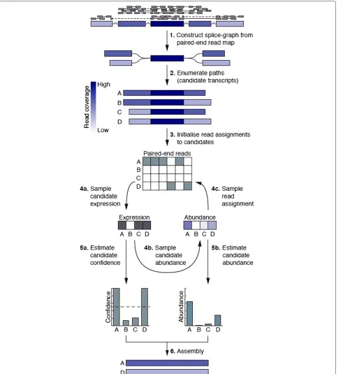
The Bayesembler

The algorithm first constructs a set of splice graphs from aTopHat2[9] map of the RNA-seq reads using the graph construction routine in the CEM [5] assembly package (Figure 1(1)). Next, for each splice graph, a set of candidate transcripts is constructed by iteratively traversing paths in the graph and pruning the edges with lowest coverage until the total number of candidates does not exceed 100 (Figure 1(2)). Provided with a set of transcript candidates, we use Bayesian inference to determine the most likely combination of candidates and corresponding abundance levels.

Our inference method is built on a generative model of the RNA sequencing process. In the model, each candi-date is associated with a binary random variable, which models whether the candidate is expressed (i.e. has non-zero abundance); this construct allows us to model our prior expectation of sparsity in the number of expressed candidates. Each expressed transcript is further associ-ated with a real-valued random variable, which models its relative abundance. Finally, we assume that the binary variables share a Bernoulli prior distribution, which con-trols the number of expressed candidates, and further

assume a symmetric Dirichlet prior distribution on the abundances of the expressed transcripts. Intuitively, this construct decouples the distribution of candidate expres-sion from the distribution over abundance levels and hereby contrasts with most current approaches by not penalising lowly abundant transcripts. To specify a com-plete generative model of the RNA sequencing process, we assume that for each transcript a binary variable is first drawn from the Bernoulli distribution, followed by a draw of abundance values from the Dirichlet distribution for the expressed transcripts. For each paired-end read to be generated, a transcript is then drawn from the categorical distribution specified by the relative abundances, followed by sampling of a paired-end read from the transcript, essentially as described by Pachter [10].

A Gibbs sampling method was derived to infer the joint posterior distribution over expressed candidates, their abundances and assignments of reads to candidate tran-scripts, where the latter represents a latent variable in our model (Figure 1(3–5)). The Gibbs sampler is initialised by randomly sampling a candidate assignment for each read and proceeds as follows (Figure 1(3)). First, candidate expression values (i.e. binary values indicating whether a transcript has non-zero abundance) are sampled con-ditioned on an assignment of reads (Figure 1(4a)). Next, abundance values are sampled conditioned on the set of expressed transcripts and read assignments (Figure 1(4b)). Finally, each read is assigned to a candidate conditioned on the expression and abundance values of all candi-dates, and the probabilities of observing the read given each of the candidates (Figure 1(4c)). The number of iterations of these three steps needed to explore the pos-terior distribution sufficiently is then calculated as an affine function of the number of candidates. The main output of the algorithm is the fraction of iterations in which a candidate transcript is expressed (our confidence metric) and a posterior mean abundance estimate for each candidate (Figure 1(5a,b)). Candidates with a con-fidence above 0.5 and at least 12 expected paired-end read counts are included in the final assembly; the lat-ter threshold is enforced to fillat-ter out putative transcript fragments (Figure 1(6)). The hyperparameter that controls the prior distribution over the number of expressed tran-scripts was estimated using a greedy minimum set cover method.

Performance evaluation

assemblers were stable and efficient enough to complete assembly on at least two of the employed datasets within a week of computation on a server with 40 CPUs. The Cufflinks, IsoLasso, CEM and Traph assemblers were selected based on these criteria. To retain a fair ground for comparison, a single set of optimalBayesembler hyper-parameters was estimated across datasets using parti-tions of the simulated, K562 and mouse dendritic cell data reserved for this purpose. Hence, the presented per-formance estimates for Bayesembler were obtained on hold-out partitions of these datasets together with the complete H1 dataset, which was reserved solely for testing purposes.

Simulated data

For the simulation study, a dataset of approximately 80 million paired-end strand-specific RNA-seq reads were simulated from the UCSC Known Genes annotation [13]

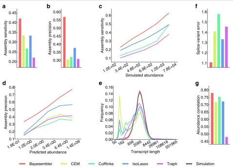
using the Flux Simulator [14]. The main measures of performance were sensitivity, defined as the fraction of simulated transcripts that were assembled correctly, and precision, defined as the fraction of assembled transcripts found in the set of simulated transcripts.

Our method exhibited both higher sensitivity and precision than all other methods (Figure 2a,b). More specifically, Bayesembler assembled 3,528 more correct transcripts, while producing 9,427 less incorrect ones on the data simulated from 40,496 annotated transcripts than the runner-up assembler,IsoLasso. Importantly, both sen-sitivity and precision remained higher for Bayesembler relative to the other assemblers independent of transcript abundance levels (Figure 2c,d). Moreover, the length dis-tribution of transcripts predicted byBayesembler resem-bled the length distribution of the simulated transcripts in contrast with the other assemblers, which tended to produce shorter transcripts (Figure 2e). Furthermore,

Bayesembler CEM Cufflinks IsoLasso Traph Simulation

d

a

b

c

e

f

g

0.45 0.50 0.55 0.60 0.65 0.70 0.75 0.80

Abundance correlation

0.30 0.35 0.40 0.45 0.50 0.55 0.60

Assembly precision

1.9E-011.2E+002.0E+003.4E+006.4E+001.4E+09 Predicted abundance 0.1

0.2 0.3 0.4 0.5 0.6 0.7 0.8

Assembly precision

1.1 1.2 1.3 1.4 1.5 1.6

Splice-variant error

0.20 0.25 0.30 0.35 0.40 0.45

Assembly sensitivity

1.2E+023.4E+024.8E+026.9E+021.2E+037.8E+04 Simulated abundance 0.1

0.2 0.3 0.4 0.5 0.6

Assembly sensitivity

50 162 6562095 8442_{26961108618551965} Transcript length

0.00 0.02 0.04 0.06 0.08 0.10 0.12 0.14 0.16

Frequency

Bayesembler was better at estimating the number of expressed splice variants for each predicted gene than the other assemblers, which may partially explain the observed improvements in assembly accuracy (Figure 2f, Figure S1 in Additional file 1). Finally, we assessed the accuracy of the transcript abundance estimates produced by the assemblers (Figure 2g, Figure S2 in Additional file 1). Here, the estimates produced by Bayesembler exhibited marginally better agreement with the simulated values compared with all other assemblers.

Real data

To assess performance on real data, the assemblers were tested on paired-end strand-specific RNA-seq data from two biological replicates from the K562 and H1 cell lines, and a single replicate of mouse dendritic cells. Impor-tantly, these datasets represent different species, tissues, library construction protocols and sequencing depths. Of note, it was not possible to run the Traph assem-bler on the K562 and H1 data due to instability of the program. As there is no gold standard transcriptome ref-erence for real data, we combined three complementary validation strategies to assess performance of the different assemblers.

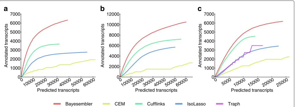
We first evaluated assembler performance by estimating the number of predicted transcripts that could be con-firmed using the UCSC Known Genes annotation against the total number of predicted transcripts. To adjust for any abundance bias in the annotation and between assem-blers, we calculated the number of confirmed transcript predictions across a sequence of thresholds on abundance and plotted it against the corresponding number of pre-dicted transcripts. Hence, the final performance metric

is a curve, where the height and slope represent sensi-tivity and precision, respectively. For both the K562 and

H1 data, the Bayesembler curve extended higher and

ascended more steeply for both replicates than any of the other assemblers thus indicating both better sensi-tivity and precision of our method (Figure 3a,b, Figure S3a,b in Additional file 1). Importantly, similar results were observed for data from mouse dendritic cells, which in turn suggests that the results are robust across species, tissues and library construction protocols (Figure 3c). Interestingly, we also observed that the transcript lengths produced byBayesemblerwere closer to the length distri-bution of annotated transcripts than the other assemblers, which again tended to produce shorter transcripts (Figure S4a–e in Additional file 1).

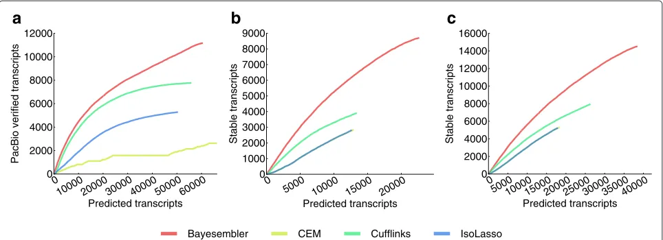
Next, we evaluated both replicate assemblies of the H1 transcriptome using data from a recent study by Au et al. [15]. In this study, RNA from the same cell line was sequenced on the Pacific Biosciences (PacBio) platform (Pacific Biosciences, California, USA), which produces significantly longer reads than standard second-generation sequencing platforms at the expense of lower throughput. As sampling bias implies that lowly abun-dant transcripts have a lower probability of being verified by a PacBio read, we again used the curve-based metric introduced above to adjust for transcript abundance bias between assemblers. Hence, we computed the number of transcript predictions that could be verified by a PacBio read against the corresponding full number of predictions across a sequence of thresholds on abundance (Figure 4a, Figure S5 in Additional file 1). In agreement with the annotation-based results,Bayesemblerfound more veri-fied transcripts both in absolute numbers and relative to

a

b

c

Bayesembler CEM Cufflinks IsoLasso Traph

0

10000 20000 30000 40000 50000 60000

Predicted transcripts 0

1000 2000 3000 4000 5000 6000 7000

Annotated transcripts

0

100002000030000400005000060000

Predicted transcripts 0

2000 4000 6000 8000 10000 12000

Annotated transcripts

0

5000 10000 15000 20000 25000

Predicted transcripts 0

1000 2000 3000 4000 5000 6000 7000

Annotated transcripts

Bayesembler CEM Cufflinks IsoLasso

a

b

c

0

100002000030000400005000060000

Predicted transcripts 0

2000 4000 6000 8000 10000 12000

PacBio verified transcripts

0

5000 10000 15000 20000

Predicted transcripts 0

1000 2000 3000 4000 5000 6000 7000 8000 9000

Stable transcripts

0

5000_{10000150002000025000300003500040000}

Predicted transcripts 0

2000 4000 6000 8000 10000 12000 14000 16000

Stable transcripts

Figure 4Assembler performance estimates for real RNA-seq data using PacBio and replicate stability-based measures.(a)The number of assembled transcripts from H1 (replicate 1) that were verified by a PacBio read against the corresponding number of predicted transcripts across a sequence of abundance thresholds (decreasing abundance threshold from left to right). The number of stable transcripts (i.e. predicted

multi-exonic transcripts that were identical between replicates) from(b)K562 and(c)H1 plotted against the corresponding number of predicted transcripts across a sequence of thresholds on transcript rank, where the ranks were obtained by sorting transcripts in each replicate in decreasing order of abundance (decreasing rank threshold from left to right).

the total number of predicted transcripts for each thresh-old, thus demonstrating better sensitivity and precision, respectively.

Finally, we leveraged the large degree of overlap expected between the transcriptomes of biological repli-cates to evaluate the different assemblers. We defined stable transcripts as multi-exonic transcripts that were present in both replicate assemblies. Again, we used a curve-based metric to correct for abundance bias between assemblers as lowly abundant transcripts are expected to be less stable. More specifically, for each pair of K562 and H1 replicates, assembled transcripts were ranked according to abundance for each of the replicates and the number of stable transcripts above a certain rank was plotted against the corresponding number of pre-dicted transcripts to produce a curve with a point for each rank (Figure 4b,c). As seen in the figure, transcripts pre-dicted byBayesemblerwere generally more stable across replicates than those of any of the other assemblers, suggesting improved performance. We further used the replicate assemblies to evaluate the impact of noise on transcript abundance estimation by comparing the esti-mates across replicates (Figures S6 and S7 in Additional file 1). Only minor differences in replicate abundance cor-relations were observed between the different assemblers, withBayesemblerperforming best for the K562 data and Cufflinksperforming best for the H1 data.

Discussion

We have devised a new probabilistic approach to tran-scriptome assembly. Our primary result is the derivation of a Bayesian model of the RNA sequencing process,

which uses a novel prior distribution over transcript abun-dances to model the number of expressed transcripts for each gene. The model thus provides a statistically consis-tent way of combininga prioriknowledge about sparsity in the number of expressed transcripts with information from the sequencing data. Importantly, in the model, only the read distribution along transcript sequences – and not transcript abundance levels – influences which transcripts are inferred as expressed. This contrasts with most cur-rent assemblers, which use abundance – either implicitly through regularisation or explicitly by truncating assem-blies at an abundance cut-off – as a proxy for transcript confidence. This is despite the fact that abundance con-tains only limited information about whether a transcript is expressed in a sample.

benchmarks suffer from the lack of a ground truth refer-ence. We therefore used a combination of simulations and three complementary metrics applied across different real datasets to gauge performance.

For simulated data, Bayesembler markedly

outper-formed all other assemblers on both sensitivity and preci-sion, withIsoLassocoming in as runner-up. Interestingly, Bayesemblerwas markedly better at estimating the num-ber of expressed transcripts for each gene, thus lending confidence to our sparsity model. In contrast, Cufflinks markedly underestimated the number of transcripts for many genes, suggesting that its strong sparsity objective negatively affects both sensitivity and precision. Real-data benchmarking was performed by comparing assem-blies with both transcript annotations, PacBio long-read sequencing data and independent assemblies made for biological replicates to adjust for biases in the individ-ual verification methods. As the latter two reference sets (and likely also annotations) all favour highly abundant transcripts, we used a novel curve-based metric to take into account any possible abundance bias between assem-blers. Bayesembler consistently outperformed all other assemblers, withCufflinkscoming in as runner-up for all metrics for all datasets. Clearly, the validity of the real-data performance metrics is strengthened because the same ranking of assembler performance was observed across metrics and datasets. The performance ranking of IsoLasso andCufflinks was inconsistent between the benchmarks for simulated and real data. We speculate that annotation-based simulations may give rise to genes with more complex splicing patterns (i.e. more variants per gene), which may have impaired the performance of Cufflinks. Abundance estimation accuracy was also investigated, with Bayesembler and Cufflinks perform-ing better than CEM and IsoLasso, but the results did not allow for performance ranking of the former two assemblers.

Importantly, the gain in accuracy provided by Bayesemblerdoes not come at the cost of increased com-putation time. Indeed, our program took approximately 5.5 hours on 16 CPU cores to assemble the deepest benchmark dataset (approximately 125 million paired-end reads) with a maximum memory footprint of 1.7 GB. This is both faster and more memory efficient than the widely usedCufflinksassembler.

Looking ahead, we believe that our method will also benefit fields outside of reference-based transcriptome assembly. First, we note that our probabilistic inference method is also directly applicable to de novoassembled splice graphs and could easily be implemented as a post-processing routine in packages likeTrinity[12] andOases [16]. Second, the ability to consistently average quantities that depend on the transcript structure provides an addi-tional advantage of our probabilistic approach. Indeed,

a recent study highlighted the influence of transcript structure on gene expression estimates [17] and we specu-late that gene expression estimates averaged across assem-blies may improve the accuracy of differential expression tests.

Conclusions

RNA-seq is rapidly becoming the de facto standard

method for expression analysis. However, despite vast amounts of available data, the reconstruction of com-plete transcripts from such data remains a fundamental challenge in computational biology.

We present hereBayesembler, a statistical approach to transcriptome assembly based on a novel Bayesian model and inference method. Using our approach, we observe a marked and consistent improvement both in bly sensitivity and precision over state-of-the-art assem-blers as judged using several independent robust measures applied across several datasets. Moreover, the use of a fully probabilistic approach allows us to provide a confidence (and an abundance) estimate for each transcript, which we expect will aid in prioritising newly discovered transcripts for experimental validation.

Materials and methods

Our transcriptome assembly algorithm proceeds by first constructing a set of splice graphs [1] (i.e. a directed acyclic graph where vertices represent exons and edges represent exon–exon junctions) from an alignment of RNA-seq reads. Next, for each splice graph, transcript candidates are enumerated by exhaustively searching paths in the graph. Bayesian inference is then used to identify the most probable transcript candidates and asso-ciated abundance levels given the reads using a generative model of the RNA sequencing process.

Splice graph construction and generation of transcript candidates

Provided with aTopHat2[9] alignment of RNA-seq reads, putative PCR duplicates and multimapping reads are first removed. Furthermore, only reads mapping in a proper paired-end fashion are retained. For strand-specific data, the originating strand is inferred for each paired-end read and splice graphs are constructed separately for each strand using the processsam utility from theCEM (v0.9.1) [5] transcriptome assembly package with the

A set of candidate transcripts is then generated for each splice graph using the following iterative procedure. The algorithm is first initialised with an edge-coverage threshold of one read. For each splice graph, all source-to-sink paths are then enumerated using a depth-first search until the search is complete or the number of candidates exceeds 100. In the latter case, the edge-coverage thresh-old is incremented by one and all edges with a coverage below the threshold removed from the graph; the graph-search and edge-pruning steps are iterated until the path search has been completed without exceeding the thresh-old or all edges have been removed. To model the presence of pre-mRNA in the sample, a candidate with a single exon spanning the entire genomic interval of the splice graph is included. Next, to leverage paired-end infor-mation, only candidates with paired-end read coverage across all splice junctions are retained. Finally, to improve detection of pre-mRNA material, candidates from over-lapping splice graphs are combined and the resulting candidate sets used as bases for the probabilistic inference method.

A generative model of the RNA-sequencing process

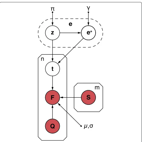
We will usesequencing fragmentto denote a read pair. The overall process of generating a setFofnsequencing frag-ments given a setSofmcandidate transcripts proceeds as follows. First, a set of relative transcript abundances tak-ing values in [0,1] is drawn from a prior distribution. The inclusion of point-zero abundances in the sample space reflects prior knowledge that only a subset of the can-didates are likely to be expressed. For each fragment to be generated, a transcript candidate is then sampled con-ditioned on the abundance values followed by sampling the fragment’s two sequencing reads conditioned on the selected candidate.

To define a prior distribution that allows for point-zero transcript abundances, let firstz be a vector of m independent random variables drawn from the Bernoulli distribution with parameterπsuch that:

P(z|π)=πbz_(1−π)m−bz_K z0

where:

bz= m

j=1

zj and Kz0 =

1 1−(1−π)m

(Supplementary methods 1 in Additional file 1). Then, let zj=0 andzj=1 indicate that transcriptsjhas point-zero

abundance (i.e.sjis not expressed) and positive abundance

(i.e.sjis expressed), respectively. Next, lete+be a vector

containing the relative abundance levels for the expressed transcripts such that:

|e+| =bz and bz

k=1 e+_k =1,

and let the values be symmetrically Dirichlet distributed such that:

P(e+|z,γ )= (bzγ ) (γ )bz

bz

k=1

e+_kγ−1

whereis the gamma function. Finally, defineeto be the vector of transcript abundances taking values in [0,1] and let it be completely specified byzande+such thatej=0

whenzj=0 andej=e+_k whenzj=1, where: k=

j

l=1 zl

Then, to generate a set of abundance values, m binary values are first drawn from the Bernoulli distribution con-ditioned on the parameterπfollowed by sampling ofe+ from the bz-dimensional symmetric Dirichlet distribu-tion. Conditioned on the set of abundances, each fragment f ∈Fis then generated by first sampling a transcript index tfrom the categorical distributionP(t|e)defined bye(i.e. P(t|e) = et). Finally, conditioned on the candidate index,

the fragment sequences are sampled fromP(f|t,q,S,μ,σ), where q ∈ Q represent the observed quality scores for fragmentf, andμandσ denote the mean and standard deviation of the fragment length distribution, respectively, essentially as proposed by Pachter [10].

The joint distribution over a set ofnfragmentsF, tran-script indicestand transcript abundanceseconditioned on the set of transcript candidates, quality scores and hyperparameters then factorises as

P(F,t,e|Q,S,μ,σ,π,γ )= P(e|π,γ )

n

i=1

Pfi|ti,qi,S,μ,σ

P(ti|e)

with

P(e|π,γ )=Pe+,z|π,γ=Pe+|z,γP(z|π) The corresponding graphical model is shown in Figure 5. Further details of the model derivation are pro-vided in Supplementary methods 1 in Additional file 1.

Approximate inference using Gibbs sampling

To apply the model to transcriptome assembly, we need to infer the posterior distribution over abundance levelse. This will in turn provide information on both whether a given transcript candidatesjis expressed (i.e. whenej>0)

Figure 5Graphical model of the joint probability distribution.

The arrows indicate dependencies between random variables. Observed and unobserved random variables are coloured inredand

white, respectively. Small filled circles indicate hyperparameters. The variables and hyperparameters are explained in the Materials and methods section and in Supplementary methods 1 in Additional file 1.

to make inference tractable, andP(t,e|F,Q,S,μ,σ,π,γ ) thus becomes the target posterior distribution. Samples from this joint distribution are obtained by iteratively drawing samples fromP(e|t,π,γ )andP(t|e,F,Q,S,μ,σ). To do this, letcdenote the vector of occurrences of each transcript index int(i.e. |c| = mandm_j=1cj = n). It

follows from the model definition that c is a sufficient statistic fortwith respect to the posterior distribution ofe. From this and our definition of the prior distribution over abundances, it follows that:

P(e|t,π,γ )=Pe+|z,c,γP(z|c,π,γ )

A sample fromP(e|t,π,γ )can then be obtained by first drawing the number of expressed transcriptsbzfrom:

P(bz|c,π,γ )=

|J0| bz− |J+|

(bzγ )

(n+bzγ )πbz(1−π)m−bz m

b=|J+|

|J0| b− |J+|

(bγ )

(n+bγ )πb(1−π)m−b where J+ is the subset of transcript indicesjfor which cj >0,J0is the subset of indices for whichcj =0 andbz is constrained such thatJ+ ≤ bz ≤ m. Conditioned on bz, a binary vectorzis first generated such thatzj=1 for

allj∈J+. The remaining transcripts are then allocated by samplingbz− |J+|transcript indicesHuniformly fromJ0 and settingz_h= 1 for allh∈H. Equivalent to the defini-tion ofe+, letc+denote the vector of occurrencescjfor

whichzj = 1. The abundance levelse+are then sampled

from:

Pe+|z,c,γ= _bz(n+bzγ )

k=1

c+_k +γ bz

k=1

e+_kc+k+γ−1

Finally, it follows from conditional independence

of the elements in t given e that a sample from

P(t|e,F,Q,S,μ,σ) can be obtained by sampling the individual elements oftfrom:

P(t|e,f,q,S,μ,σ)= P

f|t,q,S,μ,σP(t|e)

_m j=1P

f|j,q,S,μ,σPj|e The sampler is initialised by randomly sampling a frag-ment assignfrag-ment t. A detailed derivation of the Gibbs sampling updates is provided in Supplementary methods 2 in Additional file 1. To estimateπ, the minimum number of transcript candidates required to explain all paired-end readsmminis obtained using a greedy method andπ estimated using:

π = mmin m

(Supplementary methods 3 in Additional file 1). The frag-ment lengths of all paired-end reads mapping uniquely to transcripts at least 2500 nt long from single-transcript graphs are used to estimate the parameters of the Gaus-sian distribution used to model fragment lengths. To minimise the influence of outliers, we use the median and median absolute deviance as estimators of μ and σ, respectively (Supplementary methods 3 in Additional file 1). Finally, an uninformative choice ofγ = 1 corre-sponding to the uniform symmetric Dirichlet distribution is used for the prior over relative abundances. The number of burn-in iterations required for each graph is

calcu-lated as 60 × m + 1000, where m is the number of

candidates; the number of subsequent iterations (i.e. the sample size) is set to 10 times the number of burn-in iterations.

(Supplementary methods 2 in Additional file 1). The final assembly is produced by selecting all transcript candidates with a confidence above 0.5 and excluding transcripts with an expected paired-end read count below 12; the latter threshold was implemented to filter out putative transcript fragments.

Implementation and availability

The inference algorithm is implemented in C++ as a com-plete transcriptome assembly package under the name Bayesemblerand supports multi-threading. The program is freely available under the MIT licence [18]. The

algo-rithm takes a TopHat2 [9] map as input and outputs

an assembly in GTF format and is thus compatible with downstream analysis tools likeCuffDiff2[17].

Benchmarking

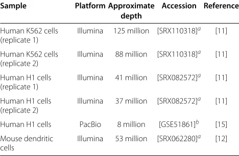
The Flux Simulator [14] (v1.2) was used to simulate approximately 80 million strand-specific paired-end reads from the human UCSC Known Genes annotation [13] (hg19 version downloaded 10 May 2013) with read lengths of 100 nt and a mean fragment length of 249 nt. Reads were simulated without variation in transcription start and end sites using the fragmentation-first protocol, where fragmentation is performed prior to reverse tran-scription with all other parameters set to their default values. Paired-end strand-specific RNA-seq data from two biological replicates of the K562 and H1 cell lines [11], and a single replicate of mouse dendritic cells [12] together with PacBio reads [15] from the H1 cell line were downloaded from the NCBI Short Read Archive and the Gene Expression Omnibus database (Table 1). Simulated and real RNA-seq reads were mapped to either the hg19 or mm10 reference genomes using Tophat2[9] (v2.0.8, default settings) together with Bowtie2 [19] (v2.1.0). The simulated, K562 and mouse data were divided into

Table 1 Datasets used in the benchmark

Sample Platform Approximate Accession Reference depth

Human K562 cells (replicate 1)

Illumina 125 million [SRX110318]a _[11]

Human K562 cells (replicate 2)

Illumina 88 million [SRX110318]a _[11]

Human H1 cells (replicate 1)

Illumina 41 million [SRX082572]a _[11]

Human H1 cells (replicate 2)

Illumina 37 million [SRX082572]a _[11]

Human H1 cells PacBio 8 million [GSE51861]b [15]

Mouse dendritic cells

Illumina 53 million [SRX062280]a [12]

a_{NCBI Sequence Read Archive.} b_{NCBI Gene Expression Omnibus.}

separatevalidation andtest sets each consisting of data from half of the chromosomes. The H1 data were reserved for testing purposes only. The validation sets were used for estimating the maximum number of candidates, how the number of Gibbs iterations should scale with the num-ber of candidates as well as the transcript confidence and expected count thresholds. Hence, the test datasets were used exclusively to produce the benchmarks presented in this paper.

The Cufflinks [2] (v2.1.1), IsoLasso [3] (v2.6), CEM [5] (v0.9.1) and Traph [8] (v0.7) assemblers were used in the performance evaluation. All assemblers were run with default parameters except that bias estimation was enabled for Cufflinks, IsoLasso andCEM, and Cufflinks was also run with multimap correction. In addition, the fragment length mean and standard deviation estimates used byBayesemblerwere provided as input toIsoLasso andCEM. Bayesembler(v1.1.1) was used in the perfor-mance evaluation.

The main benchmark criteria for the simulated data were sensitivity, defined as the fraction of simulated transcripts that were predicted correctly, and precision, defined as the fraction of predicted transcripts that were found in the simulation set. Here, a transcript match was defined as a complete intron-chain match between an assembled transcript and a simulated transcript (i.e. identical intron coordinates between the two transcripts). Single exon transcripts were considered matches if they were contained in and covered at least 75% of a sim-ulated single-exon transcript. As neitherCEM,IsoLasso nor Traphprovides full support for strand-specific data, transcripts were not matched by strand to provide a con-servative estimate of our performance relative to these assemblers. Of note, the abundance estimates of all other assemblers were renormalised to the total library size to allow for visual comparison with the Bayesembler estimates to produce Figure 2d and Figures S2, S6 and S7 in Additional file 1. Spearman’s rank correlation coef-ficient was used to assess the accuracy of the abun-dance estimates for each assembler; this metric was selected to provide robustness to the scale of abun-dances and outliers. To adjust for assembly size, only abundance values of transcripts assembled correctly by all assemblers (i.e. the intersection between assemblies and the simulation set) were used to compute the correlations.

any abundance bias in the confirmation method using the same transcript matching criteria as defined above for the simulated transcripts. The same metric was also used for further evaluation of the assemblers’ performance on the H1 datasets using PacBio reads for confirmation. Finally, performance was also estimated by assessing the over-lap between replicate assemblies from the K562 and H1 datasets. To do this, we defined stable transcripts as multi-exonic transcripts that were present in both replicate assemblies. Assembled transcripts were ranked accord-ing to abundance for each of the two replicates, and the number of stable transcripts was plotted against the corresponding number of predicted transcripts above a certain rank, thus producing a curve with a point for each rank. Finally, Spearman’s rank correlation coefficient was computed for the predicted abundances of transcripts assembled for both replicates. Only the intersection between stable transcripts of the different assemblers was used to compute the correlations to adjust for assembly size.

Additional file

Additional file 1: Supplementary information.Supplementary figures S1–S7 and Supplementary methods 1–3.

Abbreviations

PacBio, Pacific Biosciences; PCR, polymerase chain reaction; RNA-seq, RNA sequencing.

Competing interests

The authors declare that they have no competing interests.

Authors’ contributions

LM and JAS contributed equally to this work. LM, JAS and AK derived the model and inference method. LM and JAS implemented the method and performed the benchmarking. LM, JAS and AK wrote the manuscript. All authors read and approved the final manuscript.

Acknowledgements

We thank Ole Winther for his advice on the model and Jes Frellsen and Lubomir Antonov for their assistance on implementation-related issues. This work was supported by grants from the Novo Nordisk Foundation and the Danish National Advanced Technical Foundation.

Received: 24 January 2014 Accepted: 9 October 2014

References

1. Heber S, Alekseyev M, Sze S-H, Tang H, Pevzner PA:Splicing graphs and EST assembly problem.Bioinformatics (Oxford, England)2002,

18:181–188.

2. Trapnell C, Williams BA, Pertea G, Mortazavi A, Kwan G, van Baren MJ, Salzberg SL, Wold BJ, Pachter L:Transcript assembly and quantification by RNA-Seq reveals unannotated transcripts and isoform switching during cell differentiation.Nat Biotechnol2010,28:511–515. 3. Li W, Feng J, Jiang T:IsoLasso: a LASSO regression approach to

RNA-Seq based transcriptome assembly.J Comput Biol2011,

18:1693–1707.

4. Li JJ, Jiang C-R, Brown JB, Huang H, Bickel PJ:Sparse linear modeling of next-generation mRNA sequencing (RNA-Seq) data for isoform discovery and abundance estimation.Proc Nat Acad Sci USA2011,

108:19867–19872.

5. Li W, Jiang T:Transcriptome assembly and isoform expression level estimation from biased RNA-seq reads.Bioinformatics (Oxford, England)2012,28:2914–2921.

6. Mezlini AM, Smith EJ, Fiume M, Buske O, Savich G, Shah S, Aparicion S, Chiang D, Goldenberg A, Brudno M:iReckon: Simultaneous isoform discovery and abundance estimation from RNA-seq data.Genome Res2012,23:519–529.

7. Behr J, Kahles A, Zhong Y, Sreedharan VT, Drewe P, Rätsch G:MITIE: Simultaneous RNA-Seq-based transcript identification and quantification in multiple samples.Bioinformatics (Oxford, England)

2013,29:2529–2538.

8. Tomescu AI, Kuosmanen A, Rizzi R, Mäkinen V, Veli M:A novel min-cost flow method for estimating transcript expression with RNA-Seq. BMC Bioinformatics2013,14:S15.

9. Kim D, Pertea G, Trapnell C, Pimentel H, Kelley R, Salzberg SL:TopHat2: accurate alignment of transcriptomes in the presence of insertions, deletions and gene fusions.Genome Biol2013,14:R36.

10. Pachter L:Models for transcript quantification from RNA-Seq.(2011) arXiv 1104.3889v2

11. Djebali S, Davis CA, Merkel A, Dobin A, Lassmann T, Mortazavi A, Tanzer A, Lagarde J, Lin W, Schlesinger F, Xue C, Marinov GK, Khatun J, Williams BA, Zaleski C, Rozowsky J, Röder M, Kokocinski F, Abdelhamid RF, Alioto T, Antoshechkin I, Baer MT, Bar NS, Batut P, Bell K, Bell I, Chakrabortty S, Chen X, Chrast J, Curado J,et al:Landscape of transcription in human cells. Nature2012,489:101–108.

12. Grabherr MG, Haas BJ, Yassour M, Levin JZ, Thompson DA, Amit I, Adiconis X, Fan L, Raychowdhury R, Zeng Q, Chen Z, Mauceli E, Hacohen N, Gnirke A, Rhind N, di Palma F, Birren BW, Nusbaum C, Lindblad-Toh K, Friedman N, Regev A:Full-length transcriptome assembly from RNA-Seq data without a reference genome.Nat Biotechnol2011,29:644–652. 13. Meyer LR, Zweig AS, Hinrichs AS, Karolchik D, Kuhn RM, Wong M, Sloan CA,

Rosenbloom KR, Roe G, Rhead B, Raney BJ, Pohl A, Malladi VS, Li CH, Lee BT, Learned K, Kirkup V, Hsu F, Heitner S, Harte RA, Haeussler M, Guruvadoo L, Goldman M, Giardine BM, Fujita PA, Dreszer TR, Diekhans M, Cline MS, Clawson H, Barber GP,et al:The UCSC genome browser database: extensions and updates 2013.Nucleic Acids Res2013,41:D64–D69. 14. Griebel T, Zacher B, Ribeca P, Raineri E, Lacroix V, Guigó R, Sammeth M:

Modelling and simulating generic RNA-Seq experiments with the flux simulator.Nucleic Acids Res2012,40:10073–10083.

15. Au KF, Sebastiano V, Afshar PT, Durruthy JD, Lee L, Williams BA, van Bakel H, Schadt EE, Reijo-Pera RA, Underwood JG, Wong WH:Characterization of the human ESC transcriptome by hybrid sequencing.Proc Nat Acad Sci USA2013,110:E4821–E4830.

16. Schulz MH, Zerbino DR, Vingron M, Birney E:Oases: robustde novo RNA-seq assembly across the dynamic range of expression levels. Bioinformatics (Oxford, England)2012,28:1086–1092.

17. Trapnell C, Hendrickson DG, Sauvageau M, Goff L, Rinn JL, Pachter L:

Differential analysis of gene regulation at transcript resolution with RNA-seq.Nat Biotechnol2013,31:46–53.

18. Bayesembler[https://github.com/bioinformatics-centre/bayesembler] 19. Langmead B, Salzberg SL:Fast gapped-read alignment with Bowtie 2.

Nat Methods2012,9:357–359.

doi:10.1186/s13059-014-0501-4

Cite this article as:Marettyet al.:Bayesian transcriptome assembly.