Evolutionary Technique for Network Routing

Technology (IJRASET)

Evolutionary Technique for Network Routing

Yogita Bhalla1, Mr. Chirag2

Electronics and Communication Department, A.P in Electronics and Communication Department

Abstract: Applying mathematics to a problem of the real world mostly means, at first, modeling the problem mathematically, maybe with hard restrictions, idealizations, or simplifications, then solving the mathematical problem, and finally drawing conclusions about the real problem based on the solutions of the mathematical problem. Since about 60 years, a shift of paradigms has taken place in some sense; the opposite way has come into fashion. The point is that the world has done well even in times when nothing about mathematical modeling was known. The one of the alternate ways is evolutionary computation, which encompasses three main components- Evolution strategies, Genetic Algorithms and Evolution programs. One such alternative is to use a GA-based routing algorithm. GA may be used for optimization of searching process for optimum path routing in a network for optimization of both the distance and the congestion problem in a network. The proposed GA structure for the problem at hand is encoded in Matlab.

Keywords: - Genetic Algorithm, Optimization, Cross-over, Mutation, RVS, SVS, Encoding in GA.

I. INTRODUCTION

GA may be used for optimization of searching process for optimum path routing in a network for optimization of both the distance and the congestion problem in a network. The proposed GA structure for the problem at hand is encoded in Matlab. Evolutionary Computation is a rapidly expanding area of artificial intelligence research, with more than twenty international events per year and at least half a dozen journals, over a thousand EC related papers are published per year [Schwefel and Kursawe, 1998] Within EC there are three classes of EA; Evolutionary Programming, Evolution Strategies, and Genetic Algorithms. These classifications are based on the level in the hierarchy of evolution being modeled by the algorithm. Evolutionary Programming (EP) models evolution as a process of adaptive species. Evolution Strategies (ESs) models evolution as a process of the adaptive behavior of individuals. Thirdly, Genetic Algorithms (GAs) models evolution at the level of genetic chromosomes i.e. the basic instructions for making things. Evolutionary Computation (EC) is the study of computing techniques based on the guiding evolutionary principle of survival of the fittest. Evolutionary Algorithms (EAs) are powerful generic search algorithms capable of giving good solutions to complex problems. Some example areas in which EAs have been applied for problem solving and modeling include; optimization, automatic programming, machine learning, economics, immune systems, ecology, population genetics, evolution and learning, and social systems (see [Goldberg, 1989], [Ross and Corne, 1994], [Alander, 1995] and[Mitchell, 1996] for examples).

II. GENETIC ALGORITHMS: DEFINITIONS

GA’s are stochastic algorithms whose search methods model some natural phenomena: genetic inheritance and Darwinian strive for survival.

GAs are search algorithms based on the mechanics of natural selection and natural genetics. They combine survival of the fittest among string structures with a structured yet randomized information exchange to form a search algorithm with some of the innovative flair of human search.

GAs are a class of general purpose (domain independent) search methods which strike a remarkable balance between exploration and exploitation of the search space.

GAs belong to the class of probabilistic algorithms, yet they are very different from random algorithms as they combine elements of directed and stochastic search. Because of this, GAs are more robust than existing directed search methods. Another important property of such genetic-based search methods is that they maintain a population of potential solutions - all other methods process a single point of the search space.

Technology (IJRASET)

Compute initial population B0 = (b1,0, . . . , bm,0);

WHILE (stopping condition not fulfilled) DO

BEGIN

FOR i := 1 TO m DO

select an individual bi,t+1 from Bt;

FOR i := 1 TO m − 1 STEP 2 DO

IF Random[0, 1] _ pC THEN

cross bi,t+1 with bi+1,t+1;

FOR i := 1 TO m DO

eventually mutate bi,t+1;

t := t + 1

END

Selection Algorithm.

Technology (IJRASET)

Fig:-2 One Point Cross Over

Fig:-3 Two Point Cross Over

Goals of The Thesis

GA-based routing algorithm has been found to be more scalable and insensitive to variations in network topologies. However, it is also known that GA-based routing algorithm is not fast enough for real-time computation [14]. minimum spanning tree (MST) of a graph is an important concept in the communication network design and other network-related problem. Given a graph with cost (or weight) associated with each edge, the MST problem is to find a spanning tree of the graph with minimal total cost. When the graph’s edge costs are fixed and the search is unconstrained, the well-known algorithm of Krushal [12] and Prim [13] can identify MST in times that are polynomial in the number of nodes [15]. We intend to use this huge stochastic optimization tool Optimum Path Routing Problem. GA may be used for optimization of searching process for optimum path routing in a network for optimization of both the distance and the congestion problem in a network. Congestion problem in a network is not treated for in reference, which we intend to take care of in the proposed GA structure for the problem at hand. The possible optimum path is one which is having minimum distance as well as the congestion factor is to be minimized through the path, a path with less congestion but having relatively larger distance may be selected as per the objective function, which takes care of both distance as well as the congestion in the path

III. LITERATURE SURVEY

A. Traveling Salesman Problem is on of the classical optimization problem, and is similar to shortest path routing, so it is worthwhile to discuss it here. Homaifar [23] states that “one approach which would certainly find the optimal solution of any TSP is the application of exhaustive enumeration and evaluation.

B. A new genetic algorithm for the MDR problems without constraints has been developed. By transforming a network to its distance complete form, a correspondence between fixed-length binary strings in the GA and feasible solutions of the problem is established.

IV. PROPOSED SOLUTION OF ROUTING PROBLEM

The following algorithm is used to encode the proposed GA for this problem:

i) Select the nodes with their x and y coordinates and associated congestion factors.

ii) Designate initial and final nodes.

Technology (IJRASET)

iv) Evaluate the fitness of the population by the objective function, which calculates the distances between nodes from the starting node to terminating node and also sums up the congestion factors of all the nodes in the path. Objective function assigns fitness to each chromosome by way of calculating the total path distance and the total congestion factor of the path represented by the chromosome.

v) Perform roulette Wheel selection on the population.

vi) Perform crossover on the new population obtained after selection, with a probability of crossover 0.8, which may be increased or decreased for faster convergence of GA.

vi) Perform Mutation with a probability of mutation between 0.001 to 0.003. Probability of mutation may be varied for faster convergence of GA.

vi) Evaluate the fitness of the population by the objective function.

vii) Check convergence of GA, stopping citation may average fitness or predefined number of runs for the GA. If stopping criterion is met, stop the GA else go to (v), Iterations continued till stopping criterion is

met.

viii) Display the optimum path with coordinates and corresponding congestion factors of the nodes.

The possible optimum path is one which is having minimum distance as well as the congestion factor is to be minimized through the path, a path with less congestion but having relatively larger distance may be selected as per the objective function, which takes care of both distance as well as the congestion in the path.

V. RESULT

The present application of GA is programmed in MATLAB. Variable length chromosomes with real coding are used. For the particular example taken here, a population size of 10 is taken. The algorithm explained in previous section is programmed for a network of total 56 nodes. Shortest path routing is the type of routing widely used in computer networks nowadays. Even though shortest path routing algorithms are well established, other alternative methods may have their own advantages. One such alternative is to use a GA-based routing algorithm. Based on previous research, GA-based routing algorithm has been found to be more scalable and insensitive to variations in network topologies. However, it is also known that GA-based routing algorithm is not fast enough for real-time computation [14]. We intend to use this huge stochastic optimization tool Optimum Path Routing Problem. GA may be used for optimization of searching process for optimum path routing in a network for optimization of both the distance and the congestion problem in a network.

VI. IMPLIMENATION OF PROPOSED ALGORITHMS IN MATLAB

The present example is coded in Matlab. Real coding with variable length chromosomes is used. The chromosome size is variable for each chromosome and each chromosome represents a probable rout having some distance and total congestion in the path. Number of nodes is fixed in the network with each node having a congestion factor associated to it having value between 0 and 1; 0 represents a totally free node while a 1 represents a totally congested node.. The following process is used to encode the proposed GA for this problem.

A. Initialization of population

In the present example a network of 56 nodes is taken, which are assigned a congestion factor. Number of nodes is fixed in the network with each node having a congestion factor associated to it having value between 0 and 1; 0 represents a totally free node while a 1 represents a totally congested node. Select the nodes with their x and y coordinates and associated congestion factors to form a path. Designate initial and final nodes of each path same as the starting node and the terminating node, Initialize the initial population in this way, having each chromosome, with its first gene as the starting node and last gene as the terminating node, so as each chromosome represents a probable path with varying number of nodes encountered in each path.

Technology (IJRASET)

[0.0, 0.0, 0.15] [0.0, 1.0, 0.83] [0.0, 2.0, 0.25]

[0.0, 5.0, 0.10] [6.0, 2.0, 0.28] [0.0, 0.0, 0.15] [6.0, 3.0, 0.97] [0.0, 1.0, 0.83] [6.0, 5.0, 0.09] [0.0, 2.0, 0.25] [6.0, 6.0, 0.98] [0.0, 8.0, 0.62] [6.0, 7.0, 0.89] [1.0, 0.0, 0.78] [6.0, 8.0, 0.74] [1.0, 1.0, 0.98] [7.0, 0.0, 0.98] [1.0, 4.0, 0.99] [7.0, 1.0, 0.99] [1.0, 8.0, 0.97] [7.0, 2.0, 0.97] [1.0, 10.0, 0.87] [7.0, 3.0, 0.87] [2.0, 0.0, 0.88] [7.0, 6.0, 0.78] [2.0, 3.0, 0.98] [7.0, 7.0, 0.98] [2.0, 4.0, 0.99] [7.0, 8.0, 0.99] [2.0, 5.0, 0.97] [8.0, 1.0, 0.64] [2.0, 7.0, 0.02] [8.0, 3.0, 0.93] [3.0, 1.0, 0.43] [8.0, 5.0, 0.97] [3.0, 3.0, 0.92] [8.0, 7.0, 0.92] [3.0, 4.0, 0.99] [8.0, 8.0, 0.83] [3.0, 9.0, 0.75] [9.0, 0.0, 0.98] [4.0, 0.0, 0.65] [9.0, 2.0, 0.99] [4.0, 4.0, 0.13] [9.0, 3.0, 0.07] [4.0, 6.0, 0.91] [9.0, 8.0, 0.57] [4.0, 7.0, 0.95] [9.0, 9.0, 0.78] [4.0, 8.0, 0.76] [9.0, 10.0, 0.08] [4.0, 9.0, 0.83] [10.0, 2.0, 0.10] [4.0, 10.0, 0.43] [10.0, 7.0, 0.25] [5.0, 0.0, 0.68] [10.0, 1.0, 0.03] [5.0, 1.0, 0.88]

[5.0, 2.0, 0.96] [5.0, 7.0, 0.67]

Initial population is as given below(comprises of 10 chromosomes of variable lengths) Chromosome 1:

[0.0, 5.0, 0.10], [0.0, 5.0, 0.10], [4.0, 10.0, 0.43], [3.0, 4.0, 0.99],[7.0, 1.0, 0.99], [8.0, 8.0, 0.83], [9.0, 9.0, 0.78], [10.0, 2.0, 0.10].

Chromosome 2:

[0.0, 5.0, 0.10], [1.0, 1.0, 0.98], [2.0, 5.0, 0.97], [4.0, 7.0, 0.95], [9.0, 0.0, 0.98], [10.0, 2.0, 0.10].

Chromosome 3:

[0.0, 5.0, 0.10], [1.0, 10.0, 0.87], [2.0, 0.0, 0.88], [4.0, 9.0, 0.83], [5.0, 0.0, 0.68],[10.0, 2.0, 0.10]. Chromosome 4:

[0.0, 5.0, 0.10], [0.0, 8.0, 0.62], [1.0, 0.0, 0.78], [2.0, 7.0, 0.02], [3.0, 1.0, 0.43], [6.0, 8.0, 0.74], [7.0, 0.0, 0.98], [10.0, 2.0, 0.10].

Chromosome 5:

Technology (IJRASET)

Chromosome 6:

[0.0, 5.0, 0.10], [0.0, 2.0, 0.25], [1.0, 4.0, 0.99], [4.0, 6.0, 0.91], [5.0, 2.0, 0.96], [8.0, 1.0, 0.64], [10.0, 2.0, 0.10]

Chromosome 7:

[0.0, 5.0, 0.10], [2.0, 3.0, 0.98], [3.0, 9.0, 0.75], [5.0, 7.0, 0.67], [6.0, 2.0, 0.28], [8.0, 7.0, 0.92], [9.0, 2.0, 0.99], [10.0, 2.0, 0.10].

Chromosome 8:

[0.0, 5.0, 0.10], [0.0, 1.0, 0.83], [1.0, 8.0, 0.97], [4.0, 4.0, 0.13], [6.0, 3.0, 0.97], [7.0, 8.0, 0.99], [8.0, 3.0, 0.93], [9.0, 3.0, 0.07], [10.0, 2.0, 0.10].

Chromosome 9:

[0.0, 5.0, 0.10], [0.0, 0.0, 0.15], [4.0, 0.0, 0.65], [6.0, 7.0, 0.89], [7.0, 2.0, 0.97], [8.0, 5.0, 0.97], [9.0, 8.0, 0.57], [10.0, 2.0, 0.10].

Chromosome 10:

[0.0, 5.0, 0.10], [6.0, 6.0, 0.98], [7.0, 3.0, 0.87], [6.0, 5.0, 0.09], [7.0, 6.0, 0.78], [7.0, 7.0, 0.98], [10.0, 1.0, 0.03], [10.0, 2.0, 0.10]. The Network of 56 nodes for the example undertaken is given in figure--

VII. OBJECTIVE FUNCTION

Objective function calculates the distances between nodes from the starting node to terminating node and also sums up the congestion factors of all the nodes in the path. Objective function assigns fitness to each chromosome by way of calculating the total path distance and the total congestion factor of the path represented by the chromosome. GA maximizes the objective function, which is reciprocal of the total sum of distance from starting node to ending node and total congestion factor through this path.









...

.(

)

.

D

x

x

y

y

i

T



















.

...(

)

.

DF

x

x

y

y

w

C

ii

T























.

...(

)

1

2

1

y

y

w

C

iii

x

x

ObjFun















Technology (IJRASET)

VIII. OPTIMIZED PATH AND CONVERGENCE CURVE FOR GA

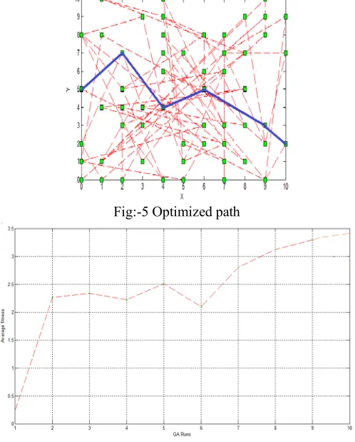
The starting node is taken as S=[0.0,5.0,0.1]; and the ending node is E=[10.0,2.0,0.1]. The Algorithm selected a path which optimizes the distance between the starting and ending node alongwith minimizing the total congestion on the path. The optimum path found by GA in present example is

S=[0.0,5.0,0.1]; [2.0,7.0,0.0]; [4.0,4.0,0.2]; [6.0,4.0,0.1]; [9.0,3.0,0.2]; E=[10.0,2.0,0.1].

The nodes are selected by the algorithm for optimizing the distance along with the congestion on the path. A shorter path with higher congestion may be neglected while longer path with lesser congestion may be selected. The path selected is shown in the figure by bold line.

GA Converges when it reaches to a optimal solution. There may be many criterions to access the convergence of GA. When the average fitness of subsequent generations stops growing then GA either converged to a optimal solution or might have struck at some suboptimal point. A predefined number of runs may be taken as the stopping criterion for the GA. Here we have tested both the stopping criterion. In this particular application fixed number of runs may be used as the optimality of the solution is visible from the output if all the chromosomes in the final population are same. The convergence curve for the GA is shown in

figure--Fig:-5 Optimized path

Fig:-6 Convergence curve for GA

IX. CONCLUSION

Technology (IJRASET)

X. FUTURE SCOPE

I tried to solve the problem for the static congestion but it can further be researched for the dynamic congestion.

REFERENCES

[1] D. E. Goldberg, Genetic Algorithms in Search, Optimization, and Machine Learning. Addison-Wesley, Reading, MA, 1989.

[2] A. Neubauer, “The circular schema theorem for genetic algorithms and two-point crossover,” in Proc. of Genetic Algorithms in Engineering Systems: Innovationsand Applications, pp. 209–214, Sept. 1997.

[3] Holland J.H. (1975) Adaptation in Natural & Artificial Systems. Ann. Arbor: The Uni. of Michigan press.

[4] Holland J.H. (1962.), “Outline for a logical theory of adaptive systems” J. Assoc. Computer. Mach., vol.3. Pp.297-314. [5] Michalewicz Z. (1992), Genetic Algorithms + Data Structures = Evolution Programs. Berlin: Springer – Verlag.

[6]Back T.(1992) “The interaction of mutation rate, selection & self adaptationin genetic algorithm,” in parallel problem solving from nature2. Manner R et.al., Eds., Amesterdam, The Neatherland: Elsevier.

[7]Back T. et.al, (1997) “Evolutionary computation: comments on the history & current state”, IEEE Transactions on Evolutionary Computations, vol 1, No. 1. [8] De Jong K. A. (1975), “An analysis of the behavior of a class of genetic adaptive system, Ph. D. Dissertation, Univ. of Michigan, Ann Arbor, Diss. Abstr. Int [9] Davis L, Ed., (1996) Handbook of Genetic Algorithms, New York: Van Norstand Reinhold.

[10] De Jong K. A. (1992), “Are Genetic Algorithms Functions Optimizers?” in Parallel Problem Solving From Nature 2. Amsterdam, the Netherlands: Elsevier. [11]Vose. M(1993), Modeling Simple Genetic Algorithms. Foundations of Genetic Algorithms -2- D. Whitley., ed., Morgan Kaufmann_ pp 63-73.

[12-8] J. B. Kruskal, “On the Shortes Spanning Tree of a Graph and the Traveling salesman Problem..” Amer. Math. Soc., vol. 7, pp. 48-50, 1956. [13] R. Prim, “Shortest Connection Networks and Some Generalization.” Bell Syst. Tech. J., vol. 36, pp. 1389-1401,1957.

[14] Salman Yousof et.al. “A Parallel Genetic Algorithm for Shortest Path Routing problem.” 2009 International Conference on Future Computer and Communication.

[15] Lixia Hanr et.al., “A Novel Genetic Algorithm for Degree-Constrained Minimum Spanning Tree Problem” IJCSNS International Journal of Computer Science and Network Security, VOL.6 No.7A, July 2006.

[17] S. Behzadi et al, “A PSEUDO GENETIC ALGORITHM FOR SOLVING BEST PATH PROBLEM.” The International Archives of the Photogrammetry, Remote Sensing and Spatial Information Sciences. Vol. XXXVII. Part B2. Beijing 2008

[18] Cauvery N K et al, “ Routing in Dynamic Network using Ants and Genetic Algorithm” IJCSNS International Journal of Computer Science and Network Security, VOL.9 No.3, March 2009

[19] Pietro Lio, Dinesh Verma, “Biologically Inspired Networking” IEEE Network • May/June 2010

[20] Salman YussofA Coarse-grained Parallel Genetic Algorithm with Migration for Shortest Path Routing Problem” 2009 11th IEEE International Conference on High Performance Computing and Communications.

[21] Edwin Núñez, “High Performance Evolutionary Computing” HPCMP Users Group Conference (HPCMP-UGC'06)0-7695-2797-3/06 $20.00 © 2006 IEEE [22]Andrew S Tannenbaum, “Computer Networks”,4th Edition, Prentice-Hall of India

[23] Abdollah Homaifar, Shanguchuan Guan, and Gunar E. Liepins. Schema analysis

of the traveling salesman problem using genetic algorithms. Complex Systems,6(2):183–217, 1992.

[24] E.L. Lawler, J.K. Lenstra, A.H.G. Rinnooy Kan, and D.B. Shmoys. The Traveling Salesman. JohnWiley and Sons, 1986. [25] Gerard Reinelt. The Traveling Salesman: Computational Solutions for TSP Applications.Springer-Verlag, 1994.

[26] Arnone S. et.al. (1994),“Toward a fuzzy government of genetic populations,” Proc.6th IEEE conf. on Tools with artificial intelligence, Los Alamitos, CA: IEEE comput. Soc. Press, pp.585-591.

[27] Bremermann,H.J (1962),“Optimization through evolution & recombination,” in Self-organizing Systems, M.C Yovits, et.al., Eds. Washington, DC, Spartan. [28] Baker J.E., (1985) “Reducing bias & inefficiency in the selection algorithm,” in Proc. 2nd _{Ann. Conf. Genetic Algorithms, Mass, Inst. Technol., Cambridge, MA,}