Comparing the ensemble and extended Kalman filters for in situ soil moisture assimilation with contrasting conditions

www.hydrol-earth-syst-sci.net/19/4811/2015/ doi:10.5194/hess-19-4811-2015

© Author(s) 2015. CC Attribution 3.0 License.

Comparing the ensemble and extended Kalman filters for

in situ soil moisture assimilation with contrasting conditions

D. Fairbairn, A. L. Barbu, J.-F. Mahfouf, J.-C. Calvet, and E. Gelati CNRM-GAME, UMR3589 – Météo-France, CNRS, Toulouse, France Correspondence to: J.-C. Calvet ([email protected])

Received: 14 June 2015 – Published in Hydrol. Earth Syst. Sci. Discuss.: 5 August 2015 Revised: 2 December 2015 – Accepted: 3 December 2015 – Published: 16 December 2015

Abstract. Two data assimilation (DA) methods are compared for their ability to produce an accurate soil moisture analysis using the Météo-France land surface model: (i) SEKF, a sim-plified extended Kalman filter, which uses a climatological background-error covariance, and (ii) EnSRF, the ensemble square root filter, which uses an ensemble background-error covariance and approximates random rainfall errors stochas-tically. In situ soil moisture observations at 5 cm depth are assimilated into the surface layer and 30 cm deep observa-tions are used to evaluate the root-zone analysis on 12 sites in south-western France (SMOSMANIA network). These sites differ in terms of climate and soil texture. The two methods perform similarly and improve on the open loop. Both meth-ods suffer from incorrect linear assumptions which are par-ticularly degrading to the analysis during water-stressed con-ditions: the EnSRF by a dry bias and the SEKF by an over-sensitivity of the model Jacobian between the surface and the root-zone layers. These problems are less severe for the sites with wetter climates. A simple bias correction technique is tested on the EnSRF. Although this reduces the bias, it mod-ifies the soil moisture fluxes and suppresses the ensemble spread, which degrades the analysis performance. However, the EnSRF flow-dependent background-error covariance ev-idently captures seasonal variability in the soil moisture er-rors and should exploit planned improvements in the model physics.

Synthetic twin experiments demonstrate that when there is only a random component in the precipitation forcing er-rors, the correct stochastic representation of these errors en-ables the EnSRF to perform better than the SEKF. It might therefore be possible for the EnSRF to perform better than the SEKF with real data, if the rainfall uncertainty was

ac-curately captured. However, the simple rainfall error model is not advantageous in our real experiments. More realistic rainfall error models are suggested.

1 Introduction

Soil moisture has a significant influence on heat and wa-ter exchanges between the land and the atmosphere, which makes it an important factor in numerical weather predic-tion (NWP) (Dharssi et al., 2011). It is also useful for a vari-ety of other applications, including drought monitoring, crop irrigation and water management.

the surface observations to the deeper layers. In situ obser-vations of root-zone soil moisture do exist, but are not dense enough over large areas.

A simplified extended Kalman filter (SEKF, Mahfouf et al., 2009) is embedded in the surface externalized (SUR-FEX) modelling platform of Météo-France (Masson et al., 2013). The SEKF simplifies the extended Kalman fil-ter (EKF) by assuming that errors in the prior state (the background) are climatological (i.e. there is no flow depen-dence in the errors) and uncorrelated between layers and grid points. The use of a linear model in the analysis up-date does extract information from the surface to the root zone. The SEKF is not yet coupled with an NWP model at Météo-France. Instead it is used to provide soil mois-ture analyses and carbon fluxes for a variety of other ap-plications, including hydrological models (see e.g. Draper et al., 2011), and the European Copernicus programme (http: //www.copernicus.eu/). An SEKF is currently coupled with the NWP model of the European Centre for Medium range Weather Forecasts (ECMWF) for the assimilation of screen-level variables (de Rosnay et al., 2013) and for the assimila-tion of ASCAT soil moisture observaassimila-tions since April 2015 (Patricia de Rosnay, personal communication). Ensemble DA methods are becoming increasingly popular for land surface models (see e.g. Reichle et al., 2002, 2008; Zhou et al., 2006; Muñoz Sabater et al., 2007; Draper et al., 2012; Carrera et al., 2015). There are four main reasons at Météo-France for de-veloping an ensemble Kalman filter (EnKF) for soil mois-ture assimilation: firstly, the EnKF uses a flow-dependent es-timate of errors in the background, rather than a climatolog-ical estimate. Secondly, the EnKF can stochastclimatolog-ically repre-sent random forcing and model errors, which is not feasible with an SEKF. Thirdly, a diffusion-based multi-layer model (Decharme et al., 2011) has been developed to replace the current three-layer force-restore land surface model. Increas-ing the number of layers would substantially increase the cost of the SEKF Jacobian calculations, which require a model in-tegration for each prognostic variable. Finally, the EnKF may take into account background-error covariances between grid points, although each grid point is assumed to be independent in this study.

The EnKF has extensively been compared with the EKF on land surface models for assimilating soil moisture obser-vations. Experiments have been conducted with both syn-thetic observations (e.g. Reichle et al., 2002) and real ob-servations (e.g. Muñoz Sabater et al., 2007). In most cases the EnKF delivered modest improvements over the EKF. It was not obvious beforehand which of these methods would perform better, since they both make incorrect linear assump-tions in the analysis update: the EKF by using a linear model and the EnKF by using a linear combination of ensemble members.

The experiments in this paper are partly motivated by studying the results of the experiments by Muñoz Sabater et al. (2007), Draper et al. (2009) and Mahfouf et al. (2009).

They performed comparisons of the SEKF and the EKF on previous versions of the land surface model used by Météo-France. They found that not only is the SEKF less computa-tionally expensive than the EKF, but that its performance is slightly better. Muñoz Sabater et al. (2007) also demonstrated that a simple 1-D variational DA method (1DVar) (theoreti-cally similar to the SEKF) performs similarly to an EnKF with a large ensemble size (≈200 members). Their results may seem counter-intuitive since the SEKF/1DVar methods cannot represent flow-dependent background errors, which can be estimated by the EKF and the EnKF. However, as the authors acknowledge, when they implemented the EKF and EnKF they did not use accurate specifications of model errors and forcing errors. The incorrect specification of these errors leads to sub-optimal filter performance (Crow and Van Loon, 2006; Reichle et al., 2008; Crow and Van den Berg, 2010).

Various formulations of the EnKF exist, which differ in the way they perform the analysis update. This study exam-ines an implementation called the ensemble square root filter (EnSRF, Whitaker and Hamill, 2002). The EnSRF is chosen because it does not perturb the observations, which would incur sampling errors. In this paper, the EnSRF is compared with the SEKF in terms of their ability to provide an accurate deterministic soil moisture analysis. The aim of this study is to compare and analyse the performances of these DA meth-ods by examining the impact of

i. random errors in the precipitation forcing;

ii. the Gaussian assumptions made by the DA methods; iii. influences of climate and soil texture; and

iv. a flow-dependent background-error covariance. A linear rescaling technique is used in this study, which bias-corrects the observations with respect to the model simula-tion (Calvet and Noilhan, 2000; Scipal et al., 2008). How-ever, ensemble perturbations can introduce additional biases as a result of the nonlinear water fluxes (Ryu et al., 2009). A simple bias correction technique is also tested on the En-SRF as a means of reducing the biases caused by ensemble perturbations (Ryu et al., 2009).

Twelve grassland sites over south-western France, where in situ observations are available (the SMOSMANIA net-work, Calvet et al., 2007; Albergel et al., 2008), are used to compare the methods. These sites include various climates and soil textures that can influence soil water transfers. In situ 5 cm deep soil moisture observations are assimilated into the surface layer. The performance is validated by comparing the root-zone soil moisture analysis (80 cm depth) with 30 cm deep in situ observations. The results are collected over a 3-year period (2008–2010).

of applying a bias correction scheme. In Sect. 3.2, the DA methods are compared using a synthetic “identical twin” ex-periment designed to represent only random errors in the precipitation forcing. This is a test of the ability of the DA methods to represent these errors. Then in Sect. 3.3 the DA methods are tested using real in situ observations. Section 4 discusses the results and Sect. 5 summarizes the main con-clusions of the experiments.

2 Methods and materials

The ISBA-A-gs model and the atmospheric forcing are intro-duced in Sects. 2.1 and 2.2 respectively. The DA methods are explained in Sect. 2.3. A list of the experiments that were per-formed is summarized in Sect. 2.4. The experimental set-ups for the real and synthetic experiments are given in Sects. 2.5 and 2.6 respectively. The experimental set-ups include a de-scription of the observations and the calibration of the error representations of the DA methods. The performance diag-nostics of the DA methods are given in Sect. 2.7.

2.1 ISBA-A-gs model

The experiments were all conducted on version 7.2 of SUR-FEX, which incorporates the Interactions between Soil, Bio-sphere and AtmoBio-sphere (ISBA) land surface model (Noilhan and Mahfouf, 1996). This model is based on the force-restore method of Deardorff (1977). The A-gs version of ISBA ac-counts for leaf-scale physiological processes, including the effects of carbon dioxide concentration and photosynthesis (Calvet et al., 1998). The simulated leaf biomass is used to compute the leaf area index (LAI), a key variable govern-ing plant transpiration. The nitrogen dilution (NIT) version of the model is applied in this work, which can dynamically simulate LAI evolution (Gibelin et al., 2006). The seasonal variability in LAI has a significant impact on the soil mois-ture variables (Barbu et al., 2011). The three-layer version of ISBA-A-gs is used in this study (Boone et al., 1999). The three soil moisture variables are defined here with the depths used for the experiments:

– the surface soil moisture (WG1), with depthd1of 1 cm. But the effective depth isd1/C1, whereC1is the surface restore coefficient, which depends on soil texture and soil moisture;

– the root-zone soil moisture (WG2), with depth d2 of 0.8 m, which includes WG1; and

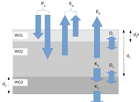
– a recharge layer (WG3) with thickness d3 of 0.2 m, which exists below WG2 (see Fig. 1).

All the variables are measured in terms of volumetric soil moisture concentration (m3m−3). A diagram illustrating the soil moisture fluxes is presented in Fig. 1. The surface layer (WG1) and the root-zone (WG2) layers are forced by

Figure 1. The soil moisture fluxes for the three-layer version of

ISBA. The variablesPg,EgandEtrrepresent the precipitation, bare soil evaporation and transpiration respectively. The fluxesKandD

represent the drainage and diffusion at the bottom of the layer.

interactions with the atmosphere and restored towards an equilibrium value. At equilibrium, the gravity forces match the capillary forces. The drainage from WG2 supplies water into a recharge zone (WG3), which conserves the total water volume.

In these experiments 12 model points were used, which are the closest points to the 12 grassland in situ observation sites (introduced in Sect. 2.5). The model points were represented by the grassland vegetation type and were located such that the nearest observation to each site was always less than 6 km away.

2.2 Forcing

The Système d’Analyse Fournissant des Renseignements à la Neige (SAFRAN) forcing was used, which is derived from a meso-scale analysis system with a horizontal resolution of 8 km (Durand et al., 1993). This provides values of precipi-tation, wind, incoming short-wave and long-wave radiation, relative humidity and air temperature, mostly derived from a surface network of weather stations. The hourly forcing values were input into the ISBA-A-gs model for the 12 grid points. We have adopted a version of SAFRAN that enables the additional use of 3000 climatological observing stations over France, including rain gauges (Quitana-Ségui et al., 2008; Vidal et al., 2010).

2.3 DA methods

xb(ti)=Mi−1 xa(ti−1)

, (1)

whereM is the (nonlinear) ISBA-A-gs model. The analysis and the observation time (ti) are at the end of the 24 h assim-ilation window. The Kalman filter analysis update is

xa(ti)=xb(ti)+Ki yoi−yi

, (2)

whereyo_{is the assimilated observation andy}

i=H (xb(ti)) is the model-predicted value of the observation (H=(1, 0) in our case). The model state and the observations are weighted using the Kalman gain (K)

Ki=BiHTi

HiBiHTi +Ri

−1

, (3)

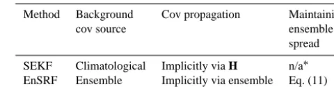
where H is the linearized observation operator, B is the background-error covariance matrix and R is the observation-error covariance matrix. These matrices mea-sure the expected errors and the covariances are a meamea-sure of the correlations in the errors between the different vari-ables (i.e. between WG1 and WG2). The R matrix is as-sumed to be diagonal, i.e. with covariances equal to zero. It is also assumed that each grid point is independent, that is, the background-error covariance is assumed to be zero between grid points. The observation is present at the end of the assimilation window, so the background-error covari-ance needs to be propagated from the beginning to the end of the window. This is implicitly calculated via H for the SEKF (Sect. 2.3.1) and via the ensemble perturbations for the En-SRF (Sect. 2.3.2). A summary of the DA methods is given in Table 1.

2.3.1 SEKF

The simplified extended Kalman filter (SEKF, Mahfouf et al., 2009) is based on the EKF (Jazwinski, 1970). The SEKF sim-plifies the EKF by using both a diagonal and climatological background-error covariance at the start of the assimilation window.

The SEKF was originally designed to assimilate screen-level temperature and humidity, which are not prognostic variables and therefore cannot be assimilated directly (Hess, 2001; Balsamo et al., 2007). For this reason the SEKF uses the linear observation operator H to relate the observed quan-tity to the prognostic variables. Following the notation of Mahfouf (2010), there are two steps in the calculation of H. The first step H1 is simply a transformation into observa-tion space (H1=(1, 0) in our case). The second step is the calculation of the tangent linear version of the nonlinear model (M). This linear model is a finite difference approx-imation between a perturbed and reference nonlinear model simulation:

Ml_i−1=Mi−1 x(ti−1)

+1x_il₋₁₋

Mi−1(x(ti−1))

1x_il₋₁ , (4)

Table 1. Table summarizing the different methods. “Cov” stands for

covariance matrix.

Method Background Cov propagation Maintaining cov source ensemble

spread SEKF Climatological Implicitly via H n/a∗ EnSRF Ensemble Implicitly via ensemble Eq. (11)

∗_{n/a=not applicable.}

where1xl is a model perturbation applied to model vari-ablel. Therefore the Jacobian between the observationkand the model variablelis simply

Hkl_i =Hk₁Ml_i−1. (5)

Equation (4) requires a model integration for each prog-nostic variable. This formulation of H implicitly prop-agates the B matrix from the start of the assimilation window to the time of the observation at the end of the window (HiBiHTi =H1Mi−1Bi−1MT_i−1HT1). Although screen-level temperature and humidity observations are not assimilated in this study, the same formulation is applied to soil moisture observations.

The 1xl size is important – it needs to be sufficiently small that the linear approximation in deriving M is satisfac-tory but large enough to not incur significant computational round-off errors. A measure of the nonlinearity of the non-linear model (M) can be calculated by the magnitude of the difference between Hkl for positive and negative values of

1xl(Walker and Houser, 2001; Balsamo et al., 2004; Draper et al., 2009), with values close to zero indicating quasi-linear model behaviour. Draper et al. (2009) and Duerinckx (2015) have demonstrated that over 6 and 24 h windows, the be-haviour of the model is generally quasi-linear for other ver-sions of ISBA. However, in both studies there were occa-sions when the model behaviour was highly nonlinear and in these situations the tangent linear approximation is inade-quate. Following Draper et al. (2009), we use a perturbation size of 10−4 _(w

fc−wwilt) and a 24 h assimilation window. Draper et al. (2009) demonstrated that during dry periods the H12 values can become much larger than 1.0, which is un-realistic and indicates highly nonlinear behaviour. For this reason we imposed a maximum limit on H12of 1.0.

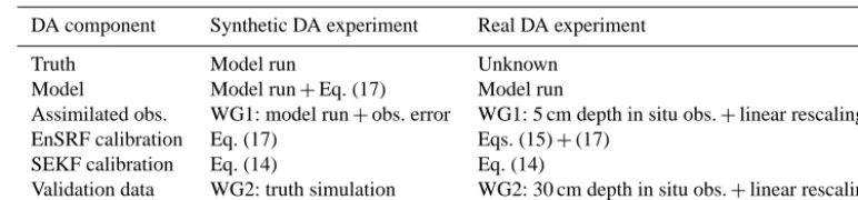
Table 2. Table showing the experimental set-up for the synthetic and real DA experiments.

DA component Synthetic DA experiment Real DA experiment

Truth Model run Unknown

Model Model run+Eq. (17) Model run

Assimilated obs. WG1: model run+obs. error WG1: 5 cm depth in situ obs.+linear rescaling EnSRF calibration Eq. (17) Eqs. (15)+(17)

SEKF calibration Eq. (14) Eq. (14)

Validation data WG2: truth simulation WG2: 30 cm depth in situ obs.+linear rescaling

KWG2=H12B

HBHT+R

−1

=H12σ_WG2b 2

H11σ_WG1b

2

+H12σ_WG2b

2

+ σo2 −1

, (6)

where σo and σb are the expected observation and back-ground errors. The R matrix in our study is equal to the scalar(σo)2.

2.3.2 EnSRF

The EnKF (Evensen, 1994) is a way of representing the un-certainty in the prognostic variables by using an ensemble of model trajectories. This circumvents the high computational cost of explicitly storing and propagating the background-error covariance for a large model dimension. First, each en-semble member is propagated using the nonlinear model:

xb_j(ti)=Mi−1

xa_j(ti−1)

, forj=1, . . ., m, (7) wheremis the ensemble size andj is the ensemble member. The following steps then occur at the analysis time (ti). The ensemble background-error covariance is defined as

Pb= 1

m−1X

b_XbT ₍₈₎

and the perturbation matrix (of dimensionn×m) is given by

Xb=√ 1

m−1

h

δxb₁. . . δxb_mi, (9)

whereδxb_j=xb_j−xbare the perturbations from the ensem-ble mean (xb) andnis the model state dimension. Note that B in Eq. (3) is expressed as Pbfor the EnSRF. The determin-istic analysis is calculated from the ensemble mean:

xa=xb+K yo−y. (10)

An additional step is required to avoid ensemble collapse. The traditional EnKF of Burgers et al. (1998) maintains the ensemble spread by perturbing the observations. The se-rial ensemble square root filter (EnSRF) was introduced by

Whitaker and Hamill (2002) as a means of avoiding the sam-pling error from the perturbed observations. The ensemble perturbations are updated by

xa_j=xa+δxb_j−αKy_j, forj=1, . . ., m, (11) where

α= 1.0

1.0+q R H Pb_HT+R

. (12)

HereRandH PbHT are scalars representing the variances at the observation location. The variable of interest WG2 is linked to WG1 via the Kalman gain:

KWG2=XbWG1

Xb_WG2

T

Xb_WG1Xb_WG1

T + σo2

−1

, (13) where XWG1XTWG2 represents the cross-product between the WG1 and WG2 ensemble perturbations. The WG1 and WG2 ensemble spreads are defined by Xb_WG1(Xb_WG1)T and Xb_WG2(Xb_WG2)T respectively.

2.4 Experiment list

The experimental set-up for the DA experiments is summa-rized in Table 2. This includes the representation of the truth, the observations, and the data used for evaluation. Descrip-tions of the real and synthetic experiments with DA are given in Sects. 2.5 and 2.6 respectively.

Table 3. Table showing the calibrations and the performances of the experiments (averaged over 2008–2010 and averaged over all sites). The

open loop is abbreviated to OL. The first two experiments were perturbed ensembles performed without DA and compared with the open loop. The synthetic and real experiments (denoted by subscripts “S” and “R”) were compared against the synthetic and real observations respectively. The variable “Pr” stands for hourly accumulated precipitation and Pr is the standard deviation of the hourly precipitation perturbation (defined in Eq. 17).

Exp. Calibration: Add. WG2 RMSE WG2 WG2 bias

Obs.λo WG1λb₁ WG2λb₂ criteria (m3m−3)×103 ACC (m3m−3)×103

Ens – – 0.025 – 9 0.97 −4.9

Ensbc – – 0.025 Bias correct 4 0.99 0.6

OLS – – – Pr=50 % Pr 2.2 0.995 0.0

EnSRFS 0.05 – – Pr=50 % Pr 1.1 0.999 0.02

SEKFS 0.05 0.04 0.02 – 1.8 0.996 0.01

OLR – – – – 24.7 0.607 0.03

EnSRF_R1 0.5 0.2 0.03 – 20.8 0.720 −5.32

EnSRFR2 0.5 0.1 0.03 Pr=50 % Pr 21.2 0.722 −5.82

EnSRF_R3 0.5 0.25 0.035 Bias correct 21.3 0.690 −2.79

SEKFR 0.5 0.25 0.25 – 20.1 0.716 −2.21

the synthetic experiments. Note that in the synthetic exper-iments, the EnSRFS was designed to capture the precipita-tion forcing uncertainty perfectly. The same precipitaprecipita-tion er-ror specification was used to estimate the precipitation erer-rors in the real experiments (EnSRFR2).

2.5 Experimental set-up: DA with real observations 2.5.1 Observations

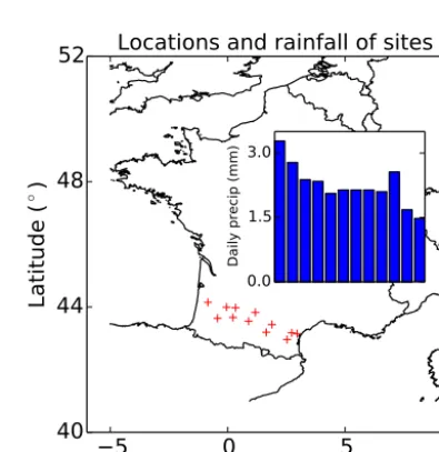
For the experiments with real observations, in situ obser-vations at 12 grassland sites in south-western France were assimilated. These experiments are hereafter referred to as “real experiments”. These grassland sites are part of the Soil Moisture Observing System Meteorological Automatic Net-work Integrated Application (SMOSMANIA) netNet-work (Cal-vet et al., 2007; Albergel et al., 2008). A map of the sites is shown in Fig. 2. Also included in Fig. 2 is a bar chart of the average daily precipitation for the sites (from west to east). The observations are spaced approximately 45 km apart. The SMOSMANIA network was selected partly be-cause of the large variability in the climatologies and soil textures between the different sites. The more westerly sites are generally wetter as they are more exposed to weather sys-tems arriving from the Atlantic Ocean. The most westerly site (Sabres) receives more than twice the average rainfall of the most easterly site (Narbonne), with a mean daily rain-fall of 3.5 mm, compared with 1.5 mm for Narbonne. Sabres also has a smaller clay to sand ratio than Narbonne. For the interested reader, Table S1.1 of the Supplement shows mod-elled and observed sand and clay percentages for each site. The larger sand particles have a smaller aggregate surface area than the finer clay particles, which means that sand can hold less water than clay. This leads to faster water transfers

5

0

5

10

Longitude (

)

40

44

48

52

La

tit

ud

e (

◦

)

Locations and rainfall of sites

0.0

1.5

3.0

Daily precip (mm)

Figure 2. Locations of the 12 sites used for the experiments (red

crosses), selected from the SMOSMANIA network. Also shown is a bar chart of the daily average rainfall for each site (plotted from west to east). The rainfall is measured from the SAFRAN forcing database over the analysis period (2008–2010).

for sandier soils. This study examines the influences of these factors on the performance of the DA methods.

depth of the layer. The observations and the model were well correlated for our experiments. The average anomaly corre-lation coefficients (ACC, defined in Sect. 2.7) for the sites between the simulated and observed WG1 (WG2) variable is 0.53 (0.68). Table S1.1 shows the WG1 and WG2 ACC for each site.

A linear rescaling technique was employed in this study, which scales the observations such that the mean and the variance match that of the model (Calvet and Noilhan, 2000; Scipal et al., 2008). The rescaling was performed over 2007– 2010. The results were calculated over 2008–2010 because a 1-year spin-up was used in the experiments. The small bias that remained, as a result of the different time periods, is not significant. There were significant biases in the in situ ob-servations (relative to the model simulation) prior to rescal-ing. The rescaling reduced the site-averaged WG1 (WG2) RMSE between the model simulation and the observations from 0.089 (0.062) to 0.060 (0.025) m3m−3_{, without} chang-ing the ACC.

It was necessary to estimate the observation errors for the DA experiments. All the ThetaProbe sensors used to measure soil moisture in the SMOSMANIA network were calibrated using gravimetric reference observations (Cal-vet et al., 2007). Overall, the RMSE after calibration was 0.038 m3m−3. This error includes instrumental errors and lo-cal representativeness errors (gravimetric samples were col-lected a few metres around the probes). However, other rep-resentativeness errors were also likely in this study, since the point observations were assumed to represent 8×8 km2 model pixels. The observation error standard deviation (σo) for WG1 was tested with values ofλo(wfc−wwilt) m3m−3, withλoequal to 0.5 or 0.35. The variableλois a dimension-less scaling coefficient for the observation error. Thewfcand

wwiltparameters are the field capacity and the wilting point respectively, and they depend on the soil texture and veg-etation type of each site. With the scaling by (wfc−wwilt) the two values of λo correspond to site-averaged σo val-ues of 0.030 and 0.044 m3m−3, which are either side of the RMSE measured by Calvet et al. (2007). The scaling by (wfc−wwilt) is based on the assumption of a linear relation-ship between the dynamic range of soil moisture values and the errors (Mahfouf et al., 2009).

2.5.2 SEKF calibration

The representation of errors by the DA methods can signif-icantly influence their performance (Reichle et al., 2008). The SEKF uses a climatological background-error covari-ance matrix. This matrix theoretically captures the total con-tribution from background errors and additive model/forcing errors. In this study, the SEKF background-error standard de-viations (σb) for WG1 and WG2 were tuned to produce the best ACC, with sizes

σ_WG1b =λb₁×(wfc−wwilt) ,

σ_WG2b =λb₂×(wfc−wwilt) . (14) In the real experiments,λb₁andλb₂were tuned between 0.0 and 0.5, in steps of 0.05. The variable λb is a dimen-sionless scaling coefficient for the calibration of the back-ground errors. The backback-ground error variances were scaled by (wfc−wwilt) for each site.

2.5.3 EnSRF calibration

The background errors in the EnSRF are implicitly captured by the ensemble spread. Hamill and Whitaker (2005) demon-strated that the addition of random perturbations to the model state (additive inflation) at the start of each cycle can be used to represent model errors. For the real experiments, Gaussian noise with zero mean and standard deviationwas added to each ensemble member after the daily analysis update. The values of for WG1 and WG2 were tuned to produce the largest ACC:

WG1=λb1×(wfc−wwilt) ,

WG2=λb2×(wfc−wwilt) , (15)

withλb₁varying between 0.0 and 0.5, in steps of 0.05, and

λb₂ varying between 0.0 and 0.05, in steps of 0.005. Time-correlated additive inflation was implemented using a first-order auto-regressive model. It was decided to use time cor-relations ofτ=1 day forWG1andτ=3 days forWG2. This is similar to previous studies (Reichle et al., 2002; Mahfouf, 2007) and is consistent with the longer time correlations of the WG2 variable compared with WG1. An ensemble size of 20 members was chosen for the calibration of the additive in-flation. The calibrated EnSRF was then tested with ensemble sizes ranging from 3 to 200 in order to explore the effects of sampling errors.

The EnSRF ensemble used hourly perturbations of the pre-cipitation forcing in order to estimate the prepre-cipitation un-certainty. The same perturbations were also used to capture precipitation errors in the synthetic experiment, and this tech-nique is described in Sect. 2.6. The performance of the En-SRF with perturbed precipitation was also compared with the performance without perturbed precipitation.

2.5.4 EnSRF bias correction

ex

b j(ti)=x

b j(ti)−x

b

j(ti)+M x a_(t

i−1),

forj =1, . . ., m, (16)

where_exb_jis the bias-correctedxb_j. Equation (16) prevents the mean of the ensemble forecasts from becoming biased with respect to the forecast of the analysis ensemble mean. The perturbation bias correction was implemented on all three layers before the analysis update step.

2.6 Experimental set-up: DA with synthetic observations

For the synthetic experiments, the in situ observations were not used, although the model was used for the same 12 sites. The truth was generated from a single model simulation. The WG1 observations were extracted from the truth with the addition of a random normally distributed observa-tion error with zero mean and standard deviaobserva-tion equal to 10 % of the higher value used in the real experiments (σo=0.05(wfc−wwilt)). The size of the observation error was small enough for the observations to have a noticeable impact on the analysis. We also tested an observation error equivalent to the value in the real experiments, and the im-pact on the analysis was about 10 times less (not shown).

A perfect model was used for the DA. However, errors were introduced in the precipitation forcing by adding ran-dom hourly perturbationsPr to the hourly precipitation ac-cumulations (Pr):

Pr∗=Pr+Pr, (17)

where Pr∗ is the perturbed hourly precipitation. The hourly perturbations were randomly sampled from a normal distri-bution with standard deviation equal to 50 % of the hourly precipitation and zero mean. The probability distribution function (pdf) was truncated in order to prevent negative val-ues of Pr∗and to maintain a mean of zero (−Pr≤Pr≤Pr). A single precipitation time series from Eq. (17) was generated over 2007–2010. This was used to force the model. A stan-dard deviation of 50 % of the hourly precipitation was judged as an appropriate order of magnitude by Reichle et al. (2002), by comparing the magnitude of the resulting errors with the difference between two precipitation data sets. Other forcing parameters were not perturbed, since it was found through a sensitivity study that perturbing these values had little im-pact on the model simulations. The results for the sensitivity study are presented in Table S1.2.

The SEKF has no means of capturing the uncertainty in the precipitation forcing from Eq. (17) directly. Therefore it was necessary to calibrate the B matrix to capture the back-ground errors that resulted from the precipitation errors. The background-error variances (σb) were calibrated with values a tenth of the values used for the real experiments (Eq. 14), since the open loop errors in the synthetic experiments were about 10 % of the errors in the real experiments.

In the synthetic experiments, the EnSRF ensemble mem-bers used the single precipitation time series from Eq. (17) to force the model. However, each ensemble member was then perturbed using Eq. (17) with different random seeds for each member. This enabled the EnSRF to capture the uncertainty in the precipitation forcing directly.

2.7 Performance diagnostics

The root mean square error (RMSE), the ACC and the bias for the WG2 variable were used to determine the perfor-mance of the DA methods:

– RMSE:

s N

P

i=0

(ye_i−H (x(ti)))2

N ;

– ACC= N

P

i=0

(H (x(ti))0−C(H (x)0))((yei)

0₋

C((ye)0))

r P

i

(H (x(ti))0−C(H (x)0))2((yei)0−C((ye)0))2 ;

– Bias: N

P

i=0

ye

i−H (x(ti))

N .

The timeti is the daily time, witht0equal to 1 January 2008 andtNequal to 31 December 2010. The climatological (time) mean ofxis defined asC(x). The observations used for eval-uation are defined as (ye_{). For the real experiments these are} in situ observations of WG2 after rescaling. In the synthetic experiments these are the true values of WG2. The anomaly

x(ti)0 is taken as the difference between the variable and a 3-month moving average.

The RMSE is a measure of both the random and system-atic components of the error. The ACC represents the sea-sonal correlations, which are unaffected by systematic errors, while the bias measures the systematic errors. The computa-tional cost of the DA methods was not assessed because the ensemble DA methods were not optimized to take advantage of parallel computing. Furthermore, Muñoz Sabater et al. (2007) already estimated the computational cost of similar algorithms on a previous version of ISBA-A-gs. They found that the main wall-clock time constraints of the EKF and EnKF algorithms were the model simulations, rather than the DA. Indeed, in our study the SEKF (which requires three simulations for the model Jacobian calculations) did have about the same wall-clock time as the EnSRF with three en-semble members.

In the experiments where DA is not applied, the perturbed model simulation is measured against the unperturbed model simulation.

3 Results

3.1 Investigating the perturbation bias (no DA)

J F M A M J J A S O N D

1.8

2.1

2.4

2.7

3.0

WG1 (mm)

(a) WG1

OL Ens Ensbc

J F M A M J J A S O N D

150

175

200

225

WG2 (mm)

(b) WG2

OL Ens Ensbc

J F M A M J J A S O N D

45

48

51

54

WG3 (mm)

(c) WG3

OL Ens Ensbc

J F M A M J J A S O N D

Month

0

20

40

60

80

100

Evapotranspiration (mm/month)

(d) Evapotranspiration

OL Ens Ensbc

J F M A M J J A S O N D

Month

0

20

40

60

80

100

Drainage (mm/month)

(e) Drainage

OL Ens Ensbc

J F M A M J J A S O N D

Month

0

8

16

24

Ens-OL (mm/month)

(f) Total depletion diff. (Ens-OL)

Ens − OL

Ensbc− OL

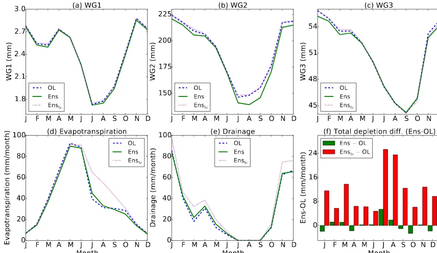
Figure 3. Monthly averaged and station-averaged net water for (a) WG1, (b) WG2 and (c) WG3 and for the open loop, the ensemble mean

(Ens) and the bias-corrected ensemble mean (Ensbc). Station-averaged and monthly (d) evapotranspiration, (e) drainage and (f) total soil water depletion differences between the ensemble mean and the open loop. Results are all averaged over the period 2008–2010.

0.025 m3m−3and zero mean. This is a similar order of mag-nitude to the values used to calibrate the ensemble spread in the real experiments (see Sect. 2.5.3). The result for the perturbed 20-member ensemble is defined as experiment Ens in Table 3. The unperturbed simulation is hereafter referred to as the open loop. The ensemble mean is compared with the open loop using the performance diagnostics defined in Sect. 2.7. A bias of −4.9×10−3m3m−3 has been intro-duced. The origin of this bias is investigated by linking the physical processes that underpin the bias to changes in the ensemble spread (Sect. 3.1.1). The influences of precipita-tion and soil clay content on the bias are then explored in Sect. 3.1.2.

3.1.1 Influence of model physics

The site-averaged (averaged over the 12 stations) and time-averaged water content of the total reservoir (WG1+WG2+WG3) is 243 mm for the open loop and 239 mm for Ens. This water loss of 4 mm (of Ens compared with the open loop) represents a small fraction of the total reservoir. The impact of the perturbed ensemble on each individual layer is demonstrated by Fig. 3, which shows the monthly, annually and site-averaged net a WG1, b WG2 and c WG3 for Ens and the open loop. The net water amount represents the concentration in m3m−3for the layer scaled by the depth of the layer (in mm). The dry bias (Ens relative to the open loop) is evident in WG2 during the entire period and it peaks between July and September. There also

appears to be a dry bias in the winter in WG3, but there is no significant bias in WG1.

The seasonal water fluxes are investigated in order to ex-plain the seasonal variabilities in the bias. Water is depleted from the reservoir via either drainage, evaporation, transpi-ration or surface runoff. Surface runoff is neglected in this investigation because it is relatively small compared with the other processes. The site-averaged monthly evapotranspi-ration (evapoevapotranspi-ration+transpiration) and drainage are shown in Fig. 3d and e respectively. The bare-soil evaporation is most active during summer, which corresponds to the max-imum insolation. The transpiration is largest in spring and early summer, when the vegetation is most developed, and before the onset of water-stressed conditions in late summer. Transpiration dominates over bare-soil evaporation, since the grassland vegetation type covers 90 % of the land surface. These two processes add up to an evapotranspiration curve which peaks in May and June (Fig. 3d). In contrast to evap-otranspiration, the drainage is most active during the winter and is absent during the late summer/early autumn period (Fig. 3e), since drainage only occurs when the soil moisture is near the field capacity.

J

2009

F M A M J J A S O N D J

2010

0.05

0.10

0.15

0.20

0.25

0.30

0.35

W

G2

(m

3

/m

3

)

Ens members Open loop Ens mean Wilting point Field capacity

J

2009

F M A M J J A S O N D J

2010

0.05

0.10

0.15

0.20

0.25

0.30

0.35

EnSRFR1 members Open loop EnSRFR1 mean Observations Wilting point Field capacity

J

2009

F M A M J J A S O N D J

2010

Time

0.05

0.10

0.15

0.20

0.25

0.30

0.35

W

G2

(m

3

/m

3

)

J

2009

F M A M J J A S O N D J

2010

Time

0.05

0.10

0.15

0.20

0.25

0.30

0.35

(a) Ens/WG2/SABRES

(b) Ens/WG2/NARBONNE

(c) EnSRF

(d) EnSRF

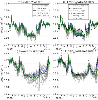
Figure 4. WG2 ensemble members, open loop and the ensemble mean for sites (top panels) Sabres and (bottom panels) Narbonne over 2009. (a) and (b) show the results for experiment Ens (no DA), while (c) and (d) show the analysis ensemble members for the EnSRFR2experiment (with observations). The field capacity and the wilting point are also shown for each site. The legends for the upper plots apply to the lower plots.

the ensemble on drainage is a slight increase relative to the open loop between February and June (Fig. 3e). The annu-ally averaged discrepancy between the Ens and open loop total soil water depletion is about 4 mm, which accounts for the dry bias in the Ens total reservoir.

It is possible to link the seasonal changes in soil water depletion to changes in the ensemble spread. The ensemble members, ensemble mean and the open loop for 2009 are shown for the Sabres site and the Narbonne site in Fig. 4a and b, respectively. Also shown are the wilting point and the field capacity for the two sites. The larger water capac-ity of clay relative to sand explains the greater field capaccapac-ity and wilting point of Narbonne compared with Sabres. During prolonged wet periods, which tend to occur in winter, the en-semble members converge because the soil reservoir reaches the field capacity. This corresponds to a reduction in the en-semble spread. Between the spring and autumn the largest fluctuations in soil moisture occur due to changes in rainfall and insolation. During this period the soil moisture

simula-tion becomes sensitive to perturbasimula-tions in the initial condi-tions, which is reflected by the large WG2 ensemble spread. The Narbonne soil has a much larger ensemble spread than the Sabres soil, particularly in autumn. Separate experiments have confirmed that this is related to the larger precipitation of Sabres compared with Narbonne, which acts to suppress the ensemble spread (see Sect. 3.1.2).

evapotran-Jun

2009

Jul

Aug

Sep

0.12

0.14

0.16

0.18

0.20

0.22

W

G2

(

m

3

/m

)

(a) Ens/WG2/NARBONNE

Ens members Open loop Ens mean Wilting point

Feb

2009

Mar

0.16

0.20

0.24

0.28

0.32

W

G2

(

m

3

/m

)

(c) Ens/WG2/NARBONNE

Ens members Open loop Ens mean Wilting point Field capacity

Jun

2009

Jul

Aug

Sep

Time

0

2

4

6

Evapotranspiration (mm/day)

(b) Ens/Evapotranspiration/NARBONNE

Feb

2009

Mar

Time

0.0

1.5

3.0

4.5

6.0

Drainage (mm/day)

(d) Ens/Drainage/NARBONNE

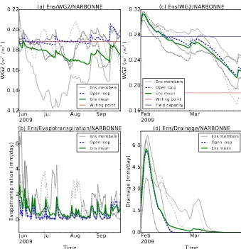
Figure 5. Four of the Ens ensemble members, open loop and the Ens ensemble mean for (a) WG2 and (b) evapotranspiration for Narbonne

between June and September 2009. (c) and (d) are equivalent to (b) and (c), but instead show WG2 and drainage respectively, for February and March 2009.

spiration for the same members is shown in Fig. 5b. The evapotranspiration is very small for the open loop and for the ensemble members below the wilting point. The members above the wilting point experience strong evapotranspiration. This effect is partly linked to the phenology; under water-stressed conditions the vegetation roots readily absorb excess water that becomes available, which increases the transpira-tion and the LAI (not shown). The Ens negative bias is larger for Narbonne than Sabres because of the greater ensemble spread for Narbonne (compare Fig. 4a with Fig. 4b).

The impact of the ensemble perturbations on drainage is most significant near the field capacity. Figure 5c and d show the soil moisture and drainage respectively for Narbonne, be-tween February and March 2009. For clarity, only five of the ensemble members are shown. When the ensemble members are greater than the field capacity, then the drainage rapidly increases, which suppresses the ensemble spread. The en-semble members below the field capacity have a drainage near zero. This implies that when the open loop is below the field capacity, and some ensemble members are above the

field capacity, the ensemble mean loses water relative to the open loop. This often occurs during the spring and autumn months, which agrees with Fig. 3e.

1.0 1.5 2.0 2.5 3.0 3.5 Mean precipitation (mm/day) 0.30

0.45 0.60 0.75 0.90

|Bias/RMSE| (-) S

N

(a) Precipitation vs bias

18 20 22 24 Clay (%) 0.30

0.45 0.60 0.75 0.90

S N

(b) Clay vs bias (Sabres forcing)

18 20 22 24 Clay (%) 0.30

0.45 0.60 0.75 0.90

S

N

(c) Clay vs bias (Narbonne forcing)

Figure 6. Average perturbation bias normalized by the RMSE against (a) average daily precipitation for each site and (b) against clay

percentage for each site, with the climatological forcing of the Sabres site applied to all the sites, and (c) same as (b) but that the climatological forcing of the Narbonne site has been applied to all the sites. The Sabres and Narbonne sites are labelled as “S” and “N” respectively. The line of best fit (linear regression) is shown for each plot.

We then performed an experiment to determine the impact of clay content on the bias. In this experiment we used the same atmospheric forcing of the wettest site (Sabres) for all the sites. This eliminates the impact of different climate on the results and leaves only differences in soil class. The clay percentage is plotted against the perturbation bias in Fig. 6b. We then repeated the experiment in Fig. 6b but instead using the same atmospheric forcing of the driest site (Narbonne) for all the sites. The results are shown in Fig. 6c. Neither Fig. 6b nor Fig. 6c shows a strong correlation between the clay percentage and the bias. On the other hand, the pertur-bation bias for the drier climate in Fig. 6c is much greater for all the sites than for the wetter climate (Fig. 6b). These results demonstrate that precipitation acts to suppress the perturba-tion bias, while clay content has little influence on the bias for these 12 sites.

3.1.3 Bias correction

The simple bias correction scheme (Eq. 16) was tested on the ensemble and the results are also shown in Table 3 (labelled as Ensbc). The bias has been reduced to less than a tenth of the size and the RMSE reduced by half compared with the original Ens. Figure 3a–c show the net soil moisture content of each layer for the bias-corrected ensemble (Ensbc). The bias correction has effectively removed the bias from all three layers.

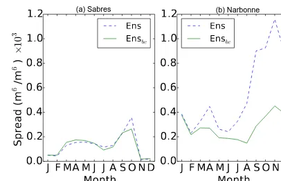
The soil water depletion is shown in Fig. 3d–f for Ensbc. It appears that the application of the bias correction scheme has inadvertently increased the soil water depletion of Ensbc relative to the open loop. A side-effect of the increase in wa-ter depletion processes is a reduction in the ensemble spread. The monthly average spread is shown in Fig. 7 for (a) Sabres and (b) Narbonne. The bias is much greater for Narbonne than Sabres (comparing Fig. 4a with Fig. 4b). Therefore the ensemble spread is halved by the bias correction for Nar-bonne, but only slightly reduced for Sabres. The reduced en-semble spread has important repercussions for DA, where the

J FMA M J J A SOND

Month

0.0

0.2

0.4

0.6

0.8

1.0

1.2

Sp

re

ad

(m

6

/m

)

×

10

3 Ens_Ens

bc

J FMA M J J A SOND

Month

0.0

0.2

0.4

0.6

0.8

1.0

1.2

Ens Ensbc

(a) Sabres (b) Narbonne

Figure 7. WG2 monthly averaged Ens and Ensbcensemble spread for (a) Sabres and (b) Narbonne. The results are averaged over 2008–2010.

ensemble spread determines the weight to give to the back-ground. This is investigated in Sect. 3.3.

3.2 SEKF vs. EnSRF: synthetic observations

The EnSRF and the SEKF were first tested with only errors in the precipitation forcing. Recall that the observations were taken from a single model simulation with a small random observation error (Sect. 2.6). For this experiment the EnSRF used a perfect stochastic representation of the precipitation uncertainty. The SEKF cannot capture the precipitation un-certainty directly, but instead the climatological background-error variances were calibrated to produce the best perfor-mance.

J F M A M J J A S O N D 0.5

1.0 1.5 2.0 2.5 3.0

RM

SE

(m

3/m

3)

×

10

3

(a) RMSE/Synthetic

OL SEKFS EnSRFS

J F M A M J J A S O N D 0.92

0.94 0.96 0.98 1.00

ACC

(b) ACC/Synthetic

OL SEKFS

EnSRFS

J F M A M J J A S O N D 0.6

0.3 0.0 0.3 0.6

Bi

as

(m

3/m

3)

×

10

3

(c) Bias/Synthetic

OL SEKFS EnSRFS

J F M A M J J A S O N D Month

10 15 20 25 30 35

RM

SE

(m

3/m 3)

×

10

3

(d) RMSE/Real

OL SEKFR EnSRFR1

J F M A M J J A S O N D Month

0.30 0.45 0.60 0.75 0.90

ACC

(e) ACC/Real

OL SEKFR EnSRFR1

J F M A M J J A S O N D Month

20 10 0 10 20

Bi

as

(m

3/m

3)

×

10

3

(f) Bias/Real

OL SEKFR EnSRFR1

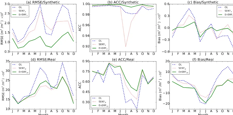
Figure 8. Site-averaged and monthly averaged (a) WG2 RMSE, (b) WG2 ACC and (c) WG2 bias for the open loop; SEKF_Sand EnSRF_S for the synthetic experiments. (d)–(f) are equivalent to (a)–(c), but instead show the results for the open loop, SEKFRand EnSRFR1for the real experiments. The results are averaged over 2008–2010.

Table 4. Site-averaged and time-averaged WG2 performances for

EnSRFS and EnSRFR1for various ensemble sizes. The calibrated EnSRF is shown in bold font.

Ens. EnSRFS EnSRFR1 EnSRFS EnSRFR1

size WG2 RMSE WG2 RMSE WG2 WG2 (m3m−3)×103 (m3m−3)×103 ACC ACC 3 1.6 24.2 1.00 0.647 6 1.4 22.5 1.00 0.687

20 1.1 20.8 1.00 0.720

50 1.1 20.9 1.00 0.719 200 1.1 20.9 1.00 0.719

ensemble sizes. The EnSRFS has an ACC close to 1.0. No significant bias was introduced because the ensemble spread was small (not shown).

The SEKFS climatological background-error covariance needed to be calibrated in order to minimize the RMSE. The SEKFSwith the optimal calibration is labelled as SEKFSin Table 3. The SEKFS performs slightly better than the open loop, but not as well as the ensemble DA methods. This is ex-pected because the SEKFSdoes not capture the uncertainty in the precipitation directly; rather, it uses larger variances in B to compensate for forcing errors. Table 5 shows the perfor-mance of the SEKFS with various background-error covari-ance specifications, with the bold font showing the optimal calibration.

The monthly average performances of the open loop and the DA methods are shown in Fig. 8a–c. The open loop RMSE is greatest in the spring and autumn seasons (Fig. 8a).

The soil moisture is going through a transition from a wet to dry state in spring and from a dry to wet state in autumn, which increases its sensitivity to perturbations in the precip-itation. During the winter the WG2 reservoir is close to the field capacity. During the summer the soil moisture is close to the wilting point and there is relatively little precipitation to perturb. Unlike the EnSRFS, the SEKFS climatological background-error covariance does not account for the sea-sonal variability in precipitation amounts. This is evidenced by examining the Kalman gains.

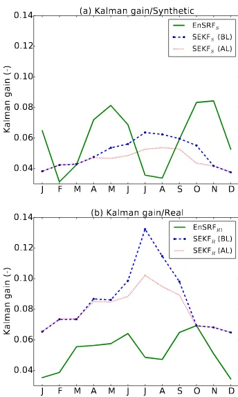
The monthly average WG2 Kalman gain for EnSRFS is displayed in Fig. 9. The EnSRFSKalman gain is closely cor-related with the open loop RMSE, with peaks in late spring and autumn. The SEKFS Kalman gain is plotted in Fig. 9 both before and after the 1.0 limit is imposed on the model Jacobian. In Sect. 2.3.1 it was explained that this limit is ex-ceeded only when the model behaviour is very nonlinear, during which time the SEKF tangent linear approximation is inadequate. In contrast to the EnSRFS Kalman gain, the SEKFS Kalman gain peaks in July. By imposing the limit on the over-sensitive Jacobian, the Kalman gain is notably reduced between May and October, which shows that the SEKFS tangent linear approximation is poor during this pe-riod. This explains why the SEKFS WG2 RMSE and ACC are worse than the open loop between June and September (Fig. 8a and b).

3.3 SEKF vs. EnSRF: real observations

perturba-J F M A M perturba-J perturba-J A S O N D 0.04

0.06 0.08 0.10 0.12 0.14

Kalman gain (-)

(a) Kalman gain/Synthetic

EnSRFS

SEKFS (BL)

SEKFS (AL)

J F M A M J J A S O N D Month

0.04 0.06 0.08 0.10 0.12 0.14

Kalman gain (-)

(b) Kalman gain/Real

EnSRFR1

SEKFR (BL)

SEKFR (AL)

Figure 9. Station and monthly averaged WG2 Kalman gains for (a) EnSRFSand the SEKFSbefore (BL) and after (AL) the Jacobian limit of 1.0 is imposed. (b) is equivalent to (a), but instead shows the results for EnSRFR1and SEKFR. The results are averaged over 2008–2010.

tions were applied to WG1 and WG2. This is labelled as EnSRFR1 in Table 3. The EnSRFR1 method does perform significantly better than the open loop (labelled as OLR in Table 3). But a dry bias has been introduced, which repre-sents a large fraction of the RMSE (25 %), and is consistent with the size of the dry bias introduced by experiment Ens in Table 3. The EnSRFR1 method was tested with various en-semble sizes and the results are shown in Table 4. There is no improvement beyond an ensemble size of 20 members.

Figure 4c and d are equivalent to Fig. 4a and b but instead show the EnSRFR1 ensemble, the open loop and the obser-vations for 2009. During December and January, the ensem-ble for Narbonne (Fig. 4d) has a similar negatively skewed spread to Fig. 4b, which indicates that the perturbation bias is present. The observations are wetter than the open loop dur-ing the summer and are therefore offsettdur-ing the perturbation bias. The opposite is true in December and January, when the observations are drier than the open loop, which causes many of the ensemble members to dip well below the wilting point. The SEKFRperformance is presented in Table 3. In terms of RMSE, SEKFRperforms marginally better than EnSRFR1, while EnSRFR1has a slightly higher ACC than SEKFR. The SEKFRmethod is also affected by a negative bias, which is

Table 5. SEKF_S performance for various calibrations of the background-error scaling coefficients (λb₁ and λb₂). The optimal value is in bold font.

λb₁ λb₂ WG2 RMSE (m3m−3)×103

0.03 0.01 2.2

0.04 0.02 1.8

0.08 0.04 2.3

0.16 0.015 2.1

about half the size of the EnSRFR1bias. The SEKFRanalysis increments themselves introduce a negative bias through the same mechanisms as the ensemble perturbation bias. But the EnSRFR1method is affected by the biases introduced by both the ensemble perturbations and the analysis increments, and therefore the EnSRFR1bias is greater than the SEKFRbias.

Figure 10 a and b show contour plots of the EnSRFR1 RMSE and ACC respectively, for the range of additive per-turbations used to calibrate the method. Figure 10 c and d show equivalent contour plots for the SEKFR. Both perfor-mance metrics are much more sensitive to the WG2 pertur-bations than the WG1 perturpertur-bations, which is logical given that the WG2 layer is much thicker than the WG1 layer. The SEKFRresults are less noisy than the EnSRFR1results (Fig. 10a and b) because the SEKF is not affected by the noise associated with the finite ensemble size of the EnSRF. The EnSRF and the SEKF were also tested with the smaller observation error of 0.35(wfc−wwilt), but this did not signif-icantly change the performance of the methods (not shown). The monthly averaged and station-averaged RMSE, the ACC and the bias are shown for the open loop, SEKFR and EnSRFR1 in Fig. 8d–f, respectively. The RMSE in all cases is highest in June and October (Fig. 8d), as this cor-responds to the greatest fluctuations in soil moisture. This is also when the most improvement over the open loop oc-curs. The EnSRFR1 RMSE is slightly degraded relative to the SEKFR in July and August as a result of the perturba-tion bias during this period (evident in Fig. 8f). The superior EnSRFR1ACC from July to September is explained below.

1

2

3

4

λ

2

(m

/m

)

10

10

20

30

40

λ

b

(m

3

/m

3

)

×

10

2

21.0

21.2

21.4

21.4

21.6 21.6

21.8 21.8

22.0

22.0 22.0

22.2

22.2

22.4

22.4

22.6 22.8 23.0

23.2

23.4

(a) EnSRF

RMSE (m

3

/m

)

₁₀

1

2

3

4

λ

2

(m

/m

)

10

10

20

30

40

λ

b

(m

3

/m

3

)

×

10

2

0.642_0.648

0.654 0.660

0.666 0.666

0.672 0.678 0.684

0.690

0.696

0.696

0.702

0.702 0.708

0.708 0.714

(b) EnSRF

ACC

10

20

30

40

λ

2

(m

/m

)

10

10

20

30

40

50

λ

b

(m

3

/m

3

)

×

10

2

20.4

20.4 20.7

20.7

21.0 21.0

21.3 21.3

21.6

21.6 21.9

21.9

22.2 22.2

22.5 22.5

22.8 22.8

23.123.4_23.7

(c) SEKF

RMSE (m

/m

)

10

10

20

30

40

λ

2

(m

/m

)

10

10

20

30

40

50

λ

b

(m

3

/m

3

)

×

10

2 0.6420.648

0.6540.6600.666

0.672

0.678

0.684 0.690

0.690 0.696

0.696 0.702 0.702

0.708

0.708

0.714

(d) SEKF

ACC

Figure 10. Contour plot showing the EnSRF_R1(a) WG2 RMSE and (b) WG2 ACC for the range of additive inflation values used to calibrate

the EnSRFR1. (c) and (d) show the equivalent contour plots to (a) and (b) for SEKFR, with the range of background-error variances used to calibrate SEKFR. The results are averaged over 2008–2010 and over the 12 sites.

The impact of precipitation forcing perturbations on the EnSRF is investigated. This experiment is labelled as EnSRFR2 in Table 3. The perturbed precipitation does not modify the analysis performance significantly compared with the unperturbed case (EnSRFR1). A slightly smaller ad-ditive inflation is optimal with the perturbed forcing. This indicates that the perturbed forcing is having a similar effect to additive covariance inflation, but without the advantages demonstrated for the idealized experiments (Sect. 3.2).

Finally, the bias correction scheme is tested on the En-SRF. This experiment is labelled “EnSRFR3” in Table 3. The large bias in Table 3 for the EnSRF without bias correc-tion (EnSRFR1) has been approximately halved by applying bias correction. The bias correction technique cannot cor-rect biases introduced by the analysis increments. Therefore EnSRFR3 is affected by a small negative bias. The ACC of EnSRFR3 is degraded relative to EnSRFR1, which is prob-ably related to unrealistic temporal changes in the ensemble spread that occur as a result of the bias correction (see Fig. 7).

4 Discussion

The discussion focusses on the knowledge gained from the experiments, referring to the four criteria set out in the intro-duction. These are the stochastic error representation of rain-fall errors (Sect. 4.1), the Gaussian assumptions (Sect. 4.2), the influence of climate and texture (Sect. 4.3), and flow de-pendence of the DA methods (Sect. 4.4). Section 4.5 dis-cusses the influence of the choice of model on the results.

4.1 Stochastic precipitation error representation

EnSRF compared with additive covariance inflation alone (compare EnSRFR2with EnSRFR1in Table 3).

Maggioni et al. (2011) demonstrated that soil moisture simulations are less sensitive to rainfall uncertainty informa-tion than the precipitainforma-tion fields themselves. They attributed this loss of information to two factors: (i) the nonlinear and integrating nature of soil moisture models; and (ii) the dis-sipative behaviour of soil moisture dynamics, which damp-ens perturbations in the initial conditions. These conclusions agree with our findings. Furthermore, the transfer of precipi-tation uncertainty information to soil moisture depends on an accurate land surface model. Significant model errors were likely in this study (see Sect. 4.5).

It is likely that the precipitation errors in this study were also underestimated. Hossain and Anagnostou (2005) esti-mated that rainfall errors represent between 20 and 60 % of the uncertainty in soil moisture prediction. In this study the estimated rainfall errors only made up 10 % of the total open loop errors. The percentage scaling in this study could not take into account the nonstationary and intermittent nature of precipitation errors, including the probability of missed precipitation or false alarms. More comprehensive precipita-tion error models have been developed which can take these factors into account (see e.g. Clark and Slater, 2006; Hos-sain and Anagnostou, 2006; Maggioni et al., 2011, 2012, 2014; Carrera et al., 2015). It is planned that one of these approaches will be adopted for the Land Data Assimilation System (LDAS) at Météo-France. The calibration of the var-ious parameters for these rainfall error models requires con-siderable testing.

4.2 Gaussian assumptions

In the synthetic experiments, the EnSRF was applied with a perfect stochastic representation of the precipitation un-certainty, while the SEKF used climatological background errors. It is possible to determine how well the DA meth-ods agreed with Kalman filter theory by comparing the pdfs of the innovations (y−yo) with the sum of the back-ground and observation-error covariances (H PbHT +R) (Desroziers et al., 2005). Figure 11 shows the histograms of the innovations normalized by

√

H Pb_HT _{+R for the} EnSRFS a and the SEKFS b for the synthetic experiments. The pdf for EnSRFS agrees very well with Kalman theory, since it has a mean of zero and it closely fits the normal dis-tribution (the green line). On the other hand, the pdf for the SEKFS is flatter than the normal distribution and therefore agrees less well with Kalman theory. This demonstrates that without the correct specification of forcing errors, the opti-mum calibration of the background-error covariance will not necessarily agree with Kalman filter theory.

In the real experiment neither method had a perfect rep-resentation of the background errors. Both methods used an average value of H PbHT +R about 4 times larger than

4 2 0 2 4

Normalized innovations 0.0

0.1 0.2 0.3 0.4

Probability

(a) Normalized innovations/EnSRFS

4 2 0 2 4

Normalized innovations 0.0

0.1 0.2 0.3 0.4

Probability

(b) Normalized innovations/SEKFS

Figure 11. Histogram of normalized innovations for the 20-member

EnSRF_S(a) and the SEKF_S(b) for the synthetic experiments. The

green line shows the normal distribution and the red dashed line shows the mean.

(y−yo)2(not shown), which indicates that the Kalman filter assumptions were incorrect.

The nonlinearity problems manifested themselves in dif-ferent ways for the SEKF and the EnSRF. For the SEKF, the Jacobian between the surface and the root zone became too large. This over-sensitivity is partly related to an unrealis-tic feature of the modelled surface energy balance, since one single surface temperature is used for bare soil and the veg-etation layer (Draper et al., 2009; Mahfouf, 2014). The En-SRF instead suffered from the perturbation bias. The expla-nation for the perturbation bias was linked to the nonlinear behaviour of evapotranspiration and drainage. Similar prob-lems were encountered by Ryu et al. (2009) on the NOAH land surface model used by the National Center for Environ-mental Prediction (NCEP), where detailed explanations are given. It should be noted that the nonlinear effects of wa-ter transfers on the ensemble perturbations are highly sensi-tive to the model and the model regime (including the layer depths and vegetation content). Indeed, Ryu et al. (2009) dis-covered a positive perturbation bias for their system, when our study discovered a negative bias.

results in inbreeding, where the errors in the background state are underestimated (Houtekamer and Mitchell, 1998). We investigated the impact of ensemble size on the EnSRF WG2 RMSE (see Table 4). It was found that sampling errors were only significant with ensemble sizes less than 20 mem-bers, which is consistent with studies by Carrera et al. (2015) and Maggioni et al. (2012). However, in all these studies the EnKF analysis is calculated independently for each grid point. It is likely that sampling errors would be much more important for a 3D-EnKF approach, where background-error covariances between grid points are taken into account, due to the much larger number of degrees of freedom.

4.3 Influences of climate and soil texture

It was discovered in Sect. 3.1.2 that there was a strong cor-relation between average precipitation and the magnitude of the perturbation bias. There are two reasons for this: firstly, the soil saturates rather quickly during precipitation events, which reduces the ensemble spread. This in turn reduces the perturbation bias. Secondly, more frequent precipitation events reduce the occurrence of ensemble members dipping below the wilting point in summer. This was confirmed by comparing the seasonal biases and the ensemble spread over the 12 sites (not shown). It is important to emphasize that these results are limited to the 12 sites, and other climate variables have not been considered.

4.4 Flow dependence

The flow dependence of the DA methods was examined by comparing the WG2 Kalman gains. When the background errors are larger, the Kalman gain should increase in order to give more weight to the observations. Given the assumption that there is no temporal evolution in the observation errors, the Kalman gain and the open loop errors should peak at the same time. In the synthetic experiments, the EnSRF Kalman gains showed a similar seasonal variability to the open loop RMSE, unlike the SEKF Kalman gains. This showed that the EnSRF was able to capture seasonal variability in the background errors. The EnSRF Kalman gains showed less seasonal variability in the real experiments, possibly because the model and forcing errors were not accurately represented. This could explain why the EnSRF performed better than the SEKF in the synthetic experiments but not in the real experi-ments.

4.5 Land surface model

In this study, the nonlinearity issues were most prevalent when the model descended below the wilting point or as-cended above the field capacity. For this reason it may seem intuitive to introduce lower and upper bounds at these thresh-olds. However, water can be slowly lost through the leaves by cuticular conductance below the wilting point or though incomplete closure of the stomata. Soil moisture may also

temporarily increase above the field capacity before it drains out (Mahfouf and Noilhan, 1996). These features are part of the NIT version of the ISBA-A-gs model. Therefore, impos-ing bounds would not be realistic. Boundary problems can also affect the analysis. For example, Ryu et al. (2009) used a bounded land surface model and found the model bounds were partly responsible for the positive perturbation bias in their study.

The SEKF and the force-restore-based ISBA-A-gs model are currently embedded in the SURFEX platform of Météo-France. However, the diffusion-based multi-layer model (ISBA-DF) will soon be implemented (Decharme et al., 2011). The soil moisture evolution of ISBA-DF is de-termined by the mixed form of the Richards equation, rather than the force-restore method. This is more realistic than the force-restore method as it solves the heat and water diffusion equations explicitly over at least five layers. Parrens et al. (2014) compared the SEKF for a 2-layer version of the force-store model with an 11-layer implementation of ISBA-DF. They found that the SEKF performance was enhanced by in-troducing multiple layers. In particular, the multi-layer model captured the vertical profile of the root-zone soil moisture better than the two-layer model. It will be interesting to test the EnSRF with ISBA-DF and multiple layers. The EnSRF flow-dependent background-error covariance may be able to exploit the improved vertical correlations between the layers.

5 Conclusions

Twelve sites in south-western France were selected for soil moisture DA experiments. The different sites were chosen, in particular, for their variability in climate and soil texture, which influence soil water transfers. The SEKF and the En-SRF DA methods were compared in terms of their ability to provide an accurate soil moisture analysis. The three-layer ISBA-A-gs land surface model (Noilhan and Mahfouf, 1996; Calvet et al., 1998) was implemented in the experiments. This model is based on the force-restore method of Deardorff (1977).