Comparison of hydrological model structures based on recession and low flow simulations

www.hydrol-earth-syst-sci.net/15/3447/2011/ doi:10.5194/hess-15-3447-2011

© Author(s) 2011. CC Attribution 3.0 License.

Earth System

Sciences

Comparison of hydrological model structures based on recession

and low flow simulations

M. Staudinger1, K. Stahl2, J. Seibert1, M. P. Clark3, and L. M. Tallaksen4

1_{Department of Geography, University of Zurich, Zurich, Switzerland}

2_{Institute of Hydrology Freiburg, Albert-Ludwigs University, Freiburg, Germany} 3_{University Cooperation for Atmospheric Research, Boulder, Colorado, USA} 4_{Department of Geosciences, University of Oslo, Oslo, Norway}

Received: 8 July 2011 – Published in Hydrol. Earth Syst. Sci. Discuss.: 13 July 2011 Revised: 27 October 2011 – Accepted: 1 November 2011 – Published: 17 November 2011

Abstract. Low flows are often poorly reproduced by

com-monly used hydrological models, which are traditionally de-signed to meet peak flow situations. Hence, there is a need to improve hydrological models for low flow prediction. This study assessed the impact of model structure on low flow simulations and recession behaviour using the Framework for Understanding Structural Errors (FUSE). FUSE identifies the set of subjective decisions made when building a hydro-logical model and provides multiple options for each mod-eling decision. Altogether 79 models were created and ap-plied to simulate stream flows in the snow dominated head-water catchment Narsjø in Norway (119 km2). All models were calibrated using an automatic optimisation method. The results showed that simulations of summer low flows were poorer than simulations of winter low flows, reflecting the importance of different hydrological processes. The model structure influencing winter low flow simulations is the lower layer architecture, whereas various model structures were identified to influence model performance during summer.

1 Motivation

Hydrological low flow periods and droughts affect water supply for drinking water, irrigation, industrial needs, hy-dropower production and ecosystems. Their occurrence is also of importance regarding environmental flow and wa-ter quality requirements, which are strongly connected to

Correspondence to: M. Staudinger ([email protected])

critical low flows (Vogel and Fennessey, 1995). Low flow and droughts affect many sectors and occur in every country albeit in different perceived severity. There is a wide range of consequences related to low flow and drought and monitor-ing and modellmonitor-ing of low flow are crucial for their analysis and prediction. However, low flows are poorly reproduced by many hydrological models since these are traditionally designed to simulate the runoff response to rainfall.

A revision of model concepts regarding low flows requires a clear understanding of the model’s structural deficits; in other words “when does it go wrong and which part of the model is the origin?” (Reusser et al., 2009). A common ap-proach to investigate the impact of the differences in model structure is to perform model intercomparison experiments (e.g. Henderson-Sellers et al., 1993; Reed et al., 2004; Duan et al., 2006; Breuer et al., 2009 and Holl¨ander et al., 2009). Such experiments have been helpful to explore model sim-ulation performance of lumped (Duan et al., 2006; Breuer et al., 2009), semi-distributed (Duan et al., 2006; Holl¨ander et al., 2009) and distributed (Henderson-Sellers et al., 1993; Reed et al., 2004; Holl¨ander et al., 2009) models in a consis-tent way using the same input data. The reasons for the ferences, however, remain unclear since each model uses dif-ferent interacting parametrisations to simulate the hydrologi-cal processes (Clark et al., 2008). Perrin et al. (2001) studied the relation between the number of optimized parameters and model performance in a multi-model, multi-catchment ex-periment, and discussed the problem of over-parametrisation and parameter uncertainty.

of the impact of the differences in model structure. Clark et al. (2008) created a computational framework that en-ables a separate evaluation of each model component. The Framework for Understanding Structural Errors (FUSE) dif-fers from others as it modularises individual flux equations instead of linking available submodels. FUSE identifies the set of subjective decisions while creating a hydrologi-cal model and offers multiple options for each model de-cision. This approach can thus help to get a better under-standing of the hydrological processes occurring. Clark et al. (2008) first introduced FUSE, as a diagnostic tool to eval-uate the performance of hydrological model structures us-ing the Nash-Sutcliffe efficiency for two climatically differ-ent catchmdiffer-ents. Clark and Kavetski (2010) evaluated several classes of numerical time stepping schemes in order to find appropriate numerical methods used to solve the governing model equations of hydrological models. The experimental setup included beside different distinct time stepping algo-rithms, eight conceptual rainfall runoff models derived from the parent models. Another recent application of FUSE is documented in the two-part series of McMillan et al. (2011) and Clark et al. (2011b). First, they used precipitation, soil moisture and streamflow data to estimate the dominant hy-drological processes of a catchment. Then, plausible repre-sentations of these processes in conceptual models were for-mulated (McMillan et al., 2011). In the second part, they evaluated FUSE models regarding their capability to simu-late those processes (Clark et al., 2011b).

Commonly, streamflow recession is modelled as the out-flow from a, or a set of, linear or non-linear reservoirs. In periods with no input, i.e. precipitation or snow melt, out-flow from the reservoirs control the streamout-flow and thus, the model behaviour during low flow. Real hydrological pro-cesses can be more complex. Therefore, it is of interest to have a closer look at the hydrograph recession, and care-fully evaluate model simulations of recession behaviour. The shape of the observed recession curve reflects the gradual de-pletion of water stored in a catchment during periods with lit-tle or no precipitation. Initially, the recession curve is steep as quick flow components like overland flow and subsurface flow contribute to streamflow. The recession curve flattens with time as e.g. delayed water from deeper subsurface stor-ages contributes, and may become nearly constant if sus-tained by outflow from the groundwater storage or from a glacier (Smakhtin, 2001). The recession curve describes in an integrated manner how different factors in a catchment influence the generation of streamflow in dry weather peri-ods (Tallaksen, 1995). Hydrogeology, relief and climate have been found to be the most important catchment properties af-fecting the recession rate (Tallaksen, 1995). Catchments with a slow recession rate are typically groundwater dominated, while impermeable catchments with little storage show faster recession rates. Moreover, summer recessions are usually faster than autumn or winter recessions (e.g. Federer, 1973; Tallaksen, 1995).

Several studies exist that link recession analysis with the structure of hydrological models (e.g. Ambroise et al., 1996; Wittenberg, 1999; Clark et al., 2009; Harman et al., 2009). In this study the model structures are systematically analysed using FUSE. The associated model performance is evaluated with respect to the ability to simulate low flows and reces-sion behaviour. This is done for one catchment only to allow a more detailed insight in the model structures. The main objective is to investigate the relative influence of a single model structure on the model performance. As there are dis-tinct differences in the recession rates found for summer and winter, one task is to study how model structure is connected to the seasonal performance for low flow simulation. This paper aims to contribute to the improvement of hydrological models for low flow prediction.

2 Data and study area

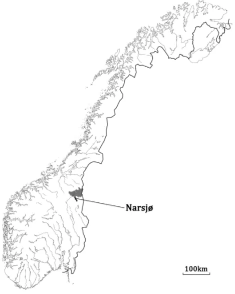
The data are from the 119 km2headwater catchment Narsjø, located in the South-East of Norway (Fig. 1) with an alti-tude range between 737 and 1595 m a.s.l. (Engeland, 2002). Narsjø is a subcatchment of the Upper Glomma basin, which is characterised by a continental climate with cold winters and relatively warm summers (Engeland, 2002). The annual snow melt flood dominates the hydrological regime. The most pronounced low flow period occurs in winter, caused by precipitation being stored in snow and ice. A second low flow period occurs in summer, caused by a lack of precipita-tion and losses due to evapotranspiraprecipita-tion (Engeland, 2002).

The geology can be divided into two main areas: one area consists of schists and phyllites that occur in combination with fine grained till soil, the other area consists of igneous rocks (granite, gneiss and gabbro) usually in combination with coarser till (Engeland, 2002). This geological charac-teristic influences the properties of soil and vegetation. The quaternary remains, consisting of several types of till and flu-vial deposits as well as bogs and lakes, form a wide, open mountain landscape with gentle slopes. The land cover is barely influenced by humans (0.3 % agricultural land) and is composed of 23.7 % forest, 60.9 % open land, 12.0 % bogs and 3.0 % lakes (Engeland, 2002).

Fig. 1. Location of the Narsjø catchment (modified after Beldring et al., 2003).

3 Methods

3.1 Snow accumulation and melt

Narsjø is a snow dominated catchment, however, there was no snow routine implemented in the version of FUSE used for this study. Hence, the input data was pre-processed with a snow accumulation and melt model. This corresponds to an implemented snow routine. Here, a simple degree day method was applied. The daily change in snow water equiva-lent1SWE [mm day−1] is equal to the difference in the daily snow accumulationas [mm day−1] and the daily snow melt ms[mm day−1] (Eq. 1).

1SWE =as −ms. (1)

The snow model separates the precipitationP [mm day−1] into rain and snow using a temperature threshold. Hence, there is only snow accumulationas in the catchment when

the measured temperatureT [◦_{C] is below the threshold}

tem-peratureTacc(Eq. 2).

as =

0, T ≥ Tacc,

P , T < Tacc. (2)

In this study Tacc was set to 1.0◦C. The daily snow

melt ms was computed (Eq. 3) with a melt factor Mf of

3.0◦_C−1_day−1 _{and a melt threshold temperature T} melt of

0◦_C.

ms =

Mf(T −Tmelt), T ≥ Tmeltand SWE > 0,

0, T < Tmeltand SWE = 0. (3)

The chosen melt factor was based on Seibert (1999) who found melt factors in Sweden to vary between 1.5 and 4◦_C−1_day−1_{, where the first value is suited for open and}

the latter for forested sites. The degree day method was ex-tended with a refreeze factorrf[−] which accounts for rain

that does not directly contribute to runoff due to the water holding capacity of an existing snow cover (Eq. 4).

P =

 



0, T ≥ Tacc,

P , T ≥TaccandP ≥ rfSWE,

(1 −rf) ms, T ≥ TaccandP < rfSWE.

(4)

3.2 FUSE framework

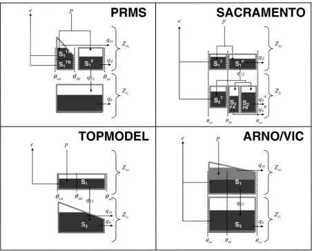
The use of FUSE as a diagnostic tool to detect the impact of model structure involved the following three steps: (1) pre-scription of the type of model (2) definition of the major model-building decisions and (3) preparation of multiple op-tions for each model building decision (Clark et al., 2008). In this study, the type of model was limited to lumped hy-drological, that were run at a daily time step (although the models are not limited to a daily time step). Four con-ceptual parent models were selected to be recombined to new FUSE-models: ARNO-VIC (Zhao, 1977), TOPMODEL (Beven and Kirkby, 1979), PRMS (Leavesley et al., 1983) and SACRAMENTO (Burnash, 1995). Simplified wiring di-agrams of the generating parent models are shown in Fig. 2. The selection of the parent FUSE models was here limited to four well known models, covering common principles used in conceptual hydrological models.

All parent models consist of equally plausible structures and the important processes could be broken down into fluxes occurring in the upper layer and lower layer, evaporation, percolation, subsurface flow and surface runoff (model build-ing options).

Fig. 2. Simplified wiring diagrams of the parent models (modified after Clark et al., 2008).

3.2.1 Upper layer

The water content of the upper soil layer was either defined as a single state variable or split into tension storage and free storage, with an additional option to further subdivide the free storage into below and above field capacity (Table 1).

3.2.2 Lower layer

The lower soil layer was either defined by a single state vari-able with unlimited storage and no lower layer evapotranspi-ration, by a single state variable with fixed storage and no lower layer evapotranspiration or as a tension storage com-bined with two parallel tanks (Table 1). All subsurface flow options (see below) are closely connected to the lower layer, this is why the choice of subsurface flow and lower-layer option is realised as a single model decision within FUSE (Clark et al., 2008).

3.2.3 Evaporation

Evaporation was parameterised by the sequential evaporation scheme (Clark et al., 2008): first potential evaporative de-mand is supplied by evaporation from the upper layer and then any residual demand by water from the lower layer.

3.2.4 Percolation

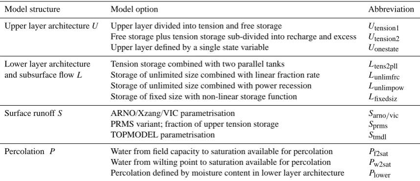
Table 1. FUSE model decision options.

Model structure Model option Abbreviation

Upper layer architectureU Upper layer divided into tension and free storage Utension1

Free storage plus tension storage sub-divided into recharge and excess Utension2

Upper layer defined by a single state variable Uonestate

Lower layer architecture Tension storage combined with two parallel tanks Ltens2pll

and subsurface flowL Storage of unlimited size combined with linear fraction rate Lunlimfrc

Storage of unlimited size combined with power recession Lunlimpow

Storage of fixed size with non-linear storage function Lfixedsiz

Surface runoffS ARNO/Xzang/VIC parametrisation Sarno/vic

PRMS variant; fraction of upper tension storage Sprms

TOPMODEL parametrisation Stmdl

Percolation P Water from field capacity to saturation available for percolation Pf2sat

Water from wilting point to saturation available for percolation Pw2sat

Percolation defined by moisture content in lower layer architecture Plower

lower layer is dry (Clark et al., 2008). All three options were used as model decision options.

3.2.5 Subsurface flow

There are four subsurface flow options (Table 1). Subsurface flow was modelled either by a single linear storage, by two parallel connected linear reservoirs or by nonlinear storage functions like in ARNO/VIC or TOPMODEL (Clark et al., 2008). TOPMODEL requires a distribution of topographic index values for each catchment (Beven and Kirkby, 1979). For the Narsjø catchment the distribution was derived using a three-parameter Gamma distribution following Sivapalan et al. (1987).

3.2.6 Surface runoff

Surface runoff was generated using a saturation-excess mechanism, when it rains on saturated areas of the basin. The surface runoff is distributed according to the topographic in-dex distribution (defined in Clark et al., 2008).

3.2.7 Bucket overflow

Additional fluxes of water may occur when one of the stor-ages reaches its capacity. In the upper layer, the bucket over-flow from the primary tension storage carries over precipi-tation that falls into the second tension storage. The bucket overflow from a tension storage carries precipitation into a free storage and from the free storage it adds to surface runoff. In the lower soil layer, the bucket overflow from tension storage forms additional percolation into free stor-age and from free storstor-age again additional subsurface flow. Following Kavetski and Kuczera (2007), logistic functions

were used to smooth the thresholds associated with a fixed capacity of model storages.

3.2.8 Routing

The time delay in runoff was modelled using a two-parameter Gamma distribution (Press et al., 1992), with an adjustable mean of the Gamma distribution. The shape of the time delay histogram, however, was fixed by setting the shape parameter to 3.0 to keep the number of adjustable parameters small.

3.3 Model calibration

All FUSE models were calibrated using the Shuffled Com-plex Evolution algorithm (SCE) which was parameterised based on the recommendations of Duan et al. (1994). A max-imum of 10 000 trials was allowed before the optimisation was terminated. Within five shuffling loops the value had to change by 10 % or the optimisation was terminated. The number of complexes in the initial population was set to 10. Each complex contained 2Nopt+ 1 points, each sub-complex Nopt+ 1 points and 2Nopt+ 1 evolution steps were allowed

for each complex before shuffling, whereNoptwas the

num-ber of parameters to be optimised in the calibration proce-dure, respectively. The algorithm was used to minimise the mean absolute relative error (FMARE) (Eq. 5).FMAREranges

between zero and infinity with the optimum at zero.

FMARE =

1

n

n X

i=1

|Qobs(i)−Qsim(i)|

Qobs(i)

3.4 Low flow and recession analysis

The performance of the model was then evaluated using the logarithmic Nash-Sutcliffe efficiency. FlogNSE was based

on log-transformed streamflow series from observationQobs

and simulationQsim(Eq. 6). This metric ranges between

mi-nus infinity and one and a perfect model would result in 1.

FlogNSE = 1 −

n P

i=1

(ln(Qobs(i)) − ln(Qsim(i)))2

n P

i=1

ln(Qobs(i)) − ln Q¯obs

2 (6)

As a good model should be able to produce reasonable re-sults for a range of objective functions the performance was evaluated usingFlogNSE, whereas the models were calibrated

usingFMARE. Calibration and validation by the two

objec-tive functions is done on the entire series, but both objecobjec-tive functions chosen emphasize the lower flow ranges of the hy-drograph.

Several studies use recession analysis to infer the exponent in a non-linear storage (Ambroise et al., 1996; Wittenberg, 1999; Clark et al., 2009; Kirchner, 2009), or, more generally, provide guidance on the structure of a hydrological model (Clark et al., 2009; Harman et al., 2009). Recession anal-ysis is also useful as a diagnostic tool for model evaluation (McMillan et al., 2011; Clark et al., 2011b). In this study the relationship between the negative change in streamflow over time−dQ

dt [mm day

−2_{] and the corresponding}

stream-flowQ[mm] was analysed using the method of Brutsaert and Nieber (1977). For the evaluation of the model performance of recessions both modelled and observed data were used. The method was modified by using flexible (instead of fixed) time steps scaled to the observed streamflow1Qbetween time steps as recommended by Rupp and Selker (2006). Our study was based on daily observations and similar to Palm-roth et al. (2010), the lower and upper limits of the time step were set to 1 and 5 days, respectively. The time step was then found by setting the maximum difference in1Q(threshold) between to time steps equal to 0.1 % of the mean observed streamflow at that point. As both−dQ

dt andQspan several

orders of magnitude, their relation is plotted in log-log-space. The data points in the plots including all recessions of the hy-drograph and might thus be composed of both subsurface and overland flow. Overland flow would mainly affect the upper range of streamflow values. Hence, the upper range in the plots of−dQ

dt andQshould be treated with special care if

interpreted regarding storage release. In case of an exponen-tial recession (simple linear storage model) the relation can be expressed as in Eq. (7), wherepis a constant. However, a power function results in Eq. (8), with the additional coef-ficientq.

dQ

dt = −p Q (7)

dQ

dt = −p Q

q ₍₈₎

The −dQ

dt versus Q plots can become noisy. Therefore,

points in a certain range of Qwere averaged to one value representative for this range (binned). Then, a polynomial function was fitted to the relationship between−dQ

dt andQ

(Eq. 9) (Kirchner, 2009). ln

_−dQ/dt

Q

≈ a +bln(Q)+c (ln(Q))2 (9)

The polynomial coefficients were fitted using a least squares regression model. The significance of the regression model was tested with the Kolmogorov-Smirnov goodness-of-fit test (Massey Jr., 1951). The polynomial fitted to the observed recessions is used as a benchmark model (see Seibert, 2001) similar to the mean streamflow being used as a benchmark model for the Nash-Sutcliffe efficiency (FNSE). Hence,

pass-ing the Kolmogorov-Smirnov test, similar to aFNSE above

zero, is used as an objective decision for acceptable mod-els (similar or better than the benchmark). The choice of a polynomial follows Kirchner (2009). It was used because of it offers both enough flexibility to adapt to the data and enough smoothness to allow moderate extrapolation beyond the binned relationships. Scatter plots of the coefficientsb

andcin Eq. (9) were then used to compare observed and sim-ulated recession behaviour for the FUSE models that passed the Kolmogorov-Smirnov goodness-of-fit test. The relation-ship between−dQ

dt andQis in the following referred to as

the “recession relationship”.

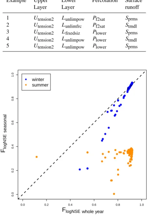
The recession behaviour was analysed for both the whole year and the individual seasons. The seasonal recessions were derived by splitting the recessions for the whole year into summer and winter recessions. Winter was defined as the time from 15 October, when precipitation generally be-gins to fall as snow in the catchment, to 15 June, which is usually towards the end of the snowmelt period.

4 Results

4.1 Calibration

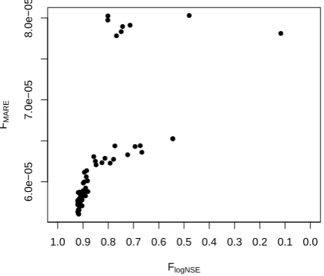
For 73 out of 79 FUSE models theFlogNSEwas greater than

zero. In Fig. 3 a scatter plot of the resulting values of the objective functions for both calibration (FMARE) and

evalua-tion (FlogNSE) is shown. The axes are ordered from high to

low model performance for both measures, which means that the points of best performance group in the lower left corner. It appears that theFlogNSE and theFMAREshow a similarly

good model performance for theFlogNSErange from 1 to 0.8.

However, for lowerFlogNSEthe two objective functions

● ●

●●

●

●● ●

● ● ●

●

● ●

●

●

●

● ●

●

● ●

●

● ● ● ●●

●

● ●●

●

● ●

●

● ●

●

● ●

● ●

● ●

● ●

● ● ● ● ●

● ●

●●●

●

● ● ●

● ●

●

● ● ● ● ● ●●● ●

FlogNSE FM

A

R

E

1.0 0.9 0.8 0.7 0.6 0.5 0.4 0.3 0.2 0.1 0.0

6.0e−05

7.0e−05

8.0e−05

Fig. 3.F_logNSEversusFMAREfor the 79 FUSE models after

cali-bration with SCE (Shuffled Complex Evolution algorithm).

4.2 Model performance during low flows

All models with FlogNSE<0 used the same

combina-tion of lower layer/subsurface flow and percolacombina-tion op-tions Lunlimpow and Plower (see Fig. 4). The best models

(FlogNSE>0.8) used varying combinations. The majority

of the best models, however, used a lower layer/subsurface flow combination of either Ltens2pll or Lfixedsiz. Many of

the poor models used a combination of Lunlimfrc for lower

layer/subsurface flow andPf2sat for percolation. The

poor-est models in the group withFlogNSE>0 primarily used the

same combination of lower layer/subsurface flow and perco-lation options as found for the poorest performing models (FlogNSE<0). All possible upper layer and surface runoff

options were found for the poorest performing models.

4.3 Recession behaviour

The observed flow values in the recession periods ranged be-tween 0.2 and 40 mm day−1for Qand between 0.001 and about 15 mm day−2for−dQ

dt and in general showed a linear

recession relationship with higher−dQ

dt for higherQ. Most

of the modelled recession relationships were similar in range, their shapes, however, differed: some appeared more con-vex, others more concave and a third group showed nearly a linear recession relationship. In comparison to the observed range, some of the models produced an unrealistic scatter. For example, low flow values were modelled that were be-low the observed range (Fig. 5f) and their associated reces-sion slopes were too steep (Fig. 5e and f). The latter be-haviour was only found for models containing a combination of the lower layer/subsurface flowLunlimpow and the

perco-lationPlower. The model decision options for the example

0.5 0.6 0.7 0.8 0.9 1.0

Lfixedsiz/Pf2sat

Lfixedsiz/Plower

Lfixedsiz/Pw2sat

Ltens2pll/Pf2sat

Ltens2pll/Plower

Ltens2pll/Pw2sat

Lunlimfrc/Pf2sat

Lunlimfrc/Plower

Lunlimfrc/Pw2sat

Lunlimpow/Pf2sat

Lunlimpow/Plower

Lunlimpow/Pw2sat

Combination lo

w

er la

y

er/percolation

FlogNSE

Fig. 4. Boxplots of the performance of models using different lower layer and percolation combinations. The box of models us-ingLunlimpowandPlowerincludes model performances (FlogNSE)

below zero.

models in Fig. 5 are listed in Table 2. The combinations including theSprmssurface runoff option (Fig. 5b, d and f)

show linear relationships, while the combinations including

Stmdl(Fig. 5c and e) show convex or concave relationships.

Figure 5e includes the lower layer/subsurface flow and per-colation optionsLunlimpowandPlowerand shows a large range

in−dQ

dt for the same flow values.

The coefficientsbandcfrom Eq. (9) are shown in Fig. 6. Thebcoefficient describes the slope and theccoefficient the curvature of the binned recession relationships. The obser-vation pair can be found at the edge of the group resulting from the simulations having a largebcoefficient and a small

ccoefficient. Most pairs are located in the lower right quar-ter, i.e. in the area of positive slope and negative curvature. A smaller group can be found for positiveb andccoefficients and only few models resulted in negativebandccoefficients. None was fitted with negative slope and positive curvature. The few models that resulted in negative slope and negative curvature usedLunlimpowfor lower layer and subsurface flow, Sprmsfor surface runoff andPlowerfor percolation.

The models that resulted in both coefficients being positive predominantly usedUonestatefor the upper layer architecture,

often combined with Lunlimfrc for lower layer/subsurface

flow. The only differing model decision option for the up-per layer architecture within this group was Utension2. All