www.hydrol-earth-syst-sci.net/16/2437/2012/ doi:10.5194/hess-16-2437-2012
© Author(s) 2012. CC Attribution 3.0 License.
Earth System
Sciences
A generic method for hydrological drought identification across
different climate regions
M. H. J. van Huijgevoort1, P. Hazenberg1,*, H. A. J. van Lanen1, and R. Uijlenhoet1
1Hydrology and Quantitative Water Management Group, Wageningen University, Wageningen, The Netherlands *now at: Department of Atmospheric Sciences, University of Arizona, Tucson, AZ, USA
Correspondence to: M. H. J. van Huijgevoort ([email protected])
Received: 25 January 2012 – Published in Hydrol. Earth Syst. Sci. Discuss.: 16 February 2012 Revised: 20 June 2012 – Accepted: 28 June 2012 – Published: 3 August 2012
Abstract. The identification of hydrological drought at global scale has received considerable attention during the last decade. However, climate-induced variation in runoff across the world makes such analyses rather complicated. This especially holds for the drier regions of the world (both cold and warm), where, for a considerable period of time, zero runoff can be observed. In the current paper, we present a method that enables to identify drought at global scale across climate regimes in a consistent manner. The method combines the characteristics of the classical variable thresh-old level method that is best applicable in regions with non-zero runoff most of the time, and the consecutive dry days (period) method that is better suited for areas where zero runoff occurs. The newly presented method allows a drought in periods with runoff to continue in the following period without runoff. The method is demonstrated by identifying droughts from discharge observations of four rivers situated within different climate regimes, as well as from simulated runoff data at global scale obtained from an ensemble of five different land surface models. The identified drought events obtained by the new approach are compared to those result-ing from application of the variable threshold level method or the consecutive dry period method separately. Results show that, in general, for drier regions, the threshold level method overestimates drought duration, because zero runoff peri-ods are included in a drought, according to the definition used within this method. The consecutive dry period method underestimates drought occurrence, since it cannot identify droughts for periods with runoff. The developed method es-pecially shows its relevance in transitional areas, because, in wetter regions, results are identical to the classical threshold level method. By combining both methods, the new method
is able to identify single drought events that occur during positive and zero runoff periods, leading to a more realis-tic global drought characterization, especially within drier environments.
1 Introduction
Climate variability causes drought to occur on all continents under all climatic conditions. Drought is one of the most costly climate-related natural hazards. The impacts are im-mense; for example, the European Commission (2007) esti-mated the total cost of droughts at C 100 billion for Europe only over the past three decades. Over the United States, the estimated damage is $ 6–8 billion per year on average (Dai, 2011). Observations show that some regions of the world (e.g. southern Europe and West Africa) have experi-enced more frequent, more intense or longer droughts, al-though in other regions the opposite happened. In the 21st century, drought is expected to intensify in some areas in Europe, Central and Northern America and Southern Africa (Seneviratne et al., 2012). Drought is one of the most imper-ative natural hazards that needs better understanding, e.g. for global food security, but receives too little attention (Romm, 2011). Lack of clarity concerning the definition of drought is one of the reasons mentioned by Seneviratne et al. (2012) for the outcome of research on historic and future drought to be presented with maximally medium confidence.
melt (meteorological drought), into the soil (soil moisture drought) and then into the aquifers, streams, lakes and reser-voirs (hydrological drought), which again can have an im-pact on local atmospheric conditions (Koster et al., 2004). This leads to socio-economic drought (impact on economic goods and services) and ecological drought (ecosystem ser-vices) (e.g. Wilhite, 2000; Tallaksen and van Lanen, 2004). Since drought is such a complex phenomenon, characterizing it requires multiple climatological and hydrological parame-ters (Mishra and Singh, 2010). Additionally, Kallis (2008) argues that interdisciplinary analyses of drought as a natu-ral hazard are needed to determine its actual impact. As a final step, policy and management options need to be iden-tified to reduce drought vulnerability, and hence the risk of future drought (e.g. Kampragou et al., 2011). For a com-plete and comprehensive assessment of drought events from the hazard to the drought management measures, the nature of each individual drought component has to be understood (Dracup et al., 1980), which urges for a step-wise approach. This paper contributes to the first step of understanding and determining the natural hazard by developing a new method-ology to identify drought. For the first time, to the authors’ knowledge, a methodology is proposed that allows identifi-cation of a drought event that starts in a period normally with runoff and continues in the period afterwards with generally no runoff in a single robust metric. Such a metric is essential, for instance, to intercompare large-scale models that have to handle very different climate conditions in one run.
Global drought studies need drought identification tools that are robust, meaning that these should be applicable to all climate regions, irrespective of the dryness of the climate. Regions with periods with and without runoff are typical for transition areas in the world, in particular from the hot and dry (hyper-arid) to the wetter climates (semi-arid) or from the extremely cold (polar frost) to the warmer climates (polar tundra). An adequate hydrological drought analysis of transi-tion areas is extremely important because of the already low water availability in normal situations (e.g. Tallaksen and van Lanen, 2004). Especially within these transitional regions, hydrological anomalies can have a dominant effect on the local climate (Koster and Suarez, 2001; Koster et al., 2004; Anyah et al., 2008), potentially intensifying the hydrological anomaly (e.g. the duration of the drought). Transition zones are also very vulnerable to climate change (e.g. Wetherald and Manabe, 2002), making projections of drought events using adequate identification tools essential. Dry areas across the world have been increasing in the last decades and will continue to increase in the future (Dai, 2011; Romm, 2011), implying that transition regions likely will move. This means that regions with zero flow will partly occur in other places, which calls for a generic method for drought analysis that can handle this non-stationary aspect of periods with and with-out runoff. When using different methods depending on re-gions, these regions might change in the future (change of periods with runoff to non-runoff periods, or the other way
around), meaning that results from different methods have to be compared for one specific period. This can be avoided by using one single all-encompassing method. A suite of identification tools has been developed to address different drought phenomena. The Standardized Precipitation Index (SPI) and the Palmer Drought Severity Index (PDSI) (e.g. Dai, 2011) are best known and widely used for large-scale studies on meteorological and soil moisture drought because of their generic applicability. The threshold level method (TLM) is another frequently applied tool for global- and continental-scale studies. For example, Sheffield and Wood (2007) used the TLM for large-scale soil moisture drought studies, and Corzo Perez et al. (2011) for drought in runoff at the global and continental scale. All these drought iden-tification tools, however, do not operate well when drought in fluxes (e.g. runoff) has to be investigated in environments where fluxes are zero for significant periods of time. Typ-ically dry regions (either hot or cold) are excluded (e.g. Corzo Perez et al., 2011), or rather high percentiles are cho-sen as threshold. For example, Fleig et al. (2006) used for a Spanish river basin a river flow that is exceeded 20 % of the time, which is not in line with the concept that drought should be uncommon. Studies in regions where precipitation is ab-sent for longer periods introduced the consecutive dry days (CDD) approach as a means to investigate variability of the length of the dry period (e.g. Vincent and Mekis, 2006; Grif-fiths and Bradley, 2007; Deni and Jemain, 2009; Im et al., 2011). In this paper, we refer to this approach as consecutive dry period method (CDPM), because it can also be applied to data with other temporal resolutions, for example monthly. So far this approach has hardly been used for ephemeral or intermittent rivers to the authors’ knowledge. Van Lanen and Tallaksen (2008) made a first attempt in two European river basins. In addition to the TLM, they identified droughts in an on-site hydrological drought analysis using the durations of months with zero flow. Nevertheless, the TLM and CDD ap-proaches were still applied separately and not combined. For droughts in runoff, one method that enables drought analysis for the whole globe is still missing. For instance, for the de-termination of synchronicity of drought at global scale, com-parison between regions is needed. This can only be achieved with a similar method across the globe.
When performing a multi-model analysis at large scale, runoff in a region might be simulated differently by each model; in particular, some models will simulate runoff and others will not for a certain region. In the case that different drought identification methods were applied to each simula-tion, model comparison would be very difficult.
A B C D E
● ●
●
●Maroni
Ashburton Ellice
[image:3.595.312.547.62.300.2]Rhine
Fig. 1. Locations of the discharge gauges of the four selected rivers within the five major climate types.
identification method combines the threshold level method and the consecutive dry period method and allows a single drought event to continue in periods with and without runoff. In this manner, new information is gained compared to ap-plying both methods separately. The presented method is pri-marily meant for natural conditions and large-scale studies, since human influences (e.g. storage dams) significantly alter flow regimes and these effects require different approaches for drought analysis as do detailed studies.
The paper starts with the main characteristics of the se-lected river basins and the land surface models (Sect. 2). The next section comprehensively elaborates step by step the drought identification approach through a description of the TLM and the CDPM, and how these eventually are integrated into a novel methodology (Sect. 3). Next, the methodology is illustrated by showing droughts in the hydrographs of the se-lected river basins, which were derived from the TLM and the CDPM separately and from the new integrated method-ology. Differences in area in drought and the average drought duration at the continental scale are used to reveal differences between the methods, as described in Sect. 4. The results are discussed in Sect. 5. Eventually, the conclusions are pre-sented (Sect. 6).
2 Data
2.1 Discharge observations across climate regimes
Observed daily discharge data of four rivers, which provide a wide range of runoff regimes, were used to illustrate the new method for hydrological drought identification. Each river is located in a different climate region (based on the K¨oppen-Geiger classification of the WATCH forcing data; see Wan-ders et al., 2010) and represents one major climate type. These five major climate types, as defined by the K¨oppen-Geiger classification, are the equatorial (A), arid (B), warm temperature (C), snow (D), and polar climates (E). These ma-jor climate types are subdivided into subtypes based on pre-cipitation regime and air temperature (Wanders et al., 2010;
1000
3000
5000
Rhine
0
2000
4000
Maroni
0
200
400
600
Ashburton
Ellice
J F M A M J J A S O N D
00
400
800
1200
Q (
m
3s
−
[image:3.595.51.287.65.189.2]1)
Fig. 2. Yearly regimes of the four selected rivers based on average daily discharge (black line) and the spread between the 10th and 90th percentile values (gray zone).
Peel et al., 2007). The four rivers selected are the Rhine (Eu-rope, C-climate), Maroni (South America, A-climate), Ash-burton (Australia, B-climate) and Ellice River (North Amer-ica, E-climate). Discharge data were made available by the Global Runoff Data Centre (GRDC, 2011). Figure 1 gives the approximate locations of the discharge gauges of these rivers. For all four rivers, their mean daily discharge regimes, as well as the spread between the 10th and 90th percentile values, are shown in Fig. 2.
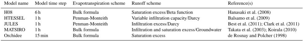
Table 1. Main characteristics of the LSMs (derived from Haddeland et al., 2011).
Model name Model time step Evapotranspiration scheme Runoff scheme Reference(s)
H08 6 h Bulk formula Saturation excess/Beta function Hanasaki et al. (2008)
HTESSEL 1 h Penman-Monteith Variable infiltration capacity/Darcy Balsamo et al. (2009)
JULES 1 h Penman-Monteith Infiltration excess/Darcy Best et al. (2011); Clark et al. (2011) MATSIRO 1 h Bulk formula Infiltration and saturation excess/Groundwater Takata et al. (2003); Koirala (2010)
Orchidee 15 min Bulk formula Saturation excess de Rosnay and Polcher (1998)
2.2 Global simulated runoff data from large-scale models
To determine drought at a global scale, generally large-scale model output is used (e.g. Sheffield and Wood, 2007). Within the EC-FP6 project WATCH (Water and Global CHange), several large-scale models have been run at global scale with the same model set-up and forcing data, described in detail by Haddeland et al. (2011).
The meteorological forcing data for the models were the WATCH forcing data (WFD) developed by Weedon et al. (2011). The WFD consist of gridded time series of meteoro-logical variables at a resolution of 0.5◦×0.5◦on a subdaily basis for the period 1958–2001. In this study, the ensemble median of results of five land surface models (LSMs) (fol-lowing the division in subgroups as proposed by Haddeland et al., 2011) was used: H08, HTESSEL, JULES, MATSIRO, Orchidee. Some model properties are given in Table 1. All models classified as LSMs by Haddeland et al. (2011) solve both the water and energy balance. The snow scheme of all models is based on the energy balance approach. They use the land mask defined by CRU (Climate Research Unit), re-sulting in a resolution of 0.5◦×0.5◦for land points only.
In large-scale climate and hydrological studies, the use of a multi-model ensemble instead of single models is quite com-mon and even advocated for simulated river flows (e.g. Stahl et al., 2012). Several studies have shown that the ensemble mean or median is often closer to the observations than ei-ther of the individual models (Gao and Dirmeyer, 2006; Guo et al., 2007; Tallaksen et al., 2011). Because this paper fo-cuses on regions with zero runoff, we have chosen to use the ensemble median instead of the mean. By taking the ensem-ble median, one model with anomalous values has less influ-ence. Some examples of time series of the ensemble median of total runoff for single grid cells, randomly chosen in dif-ferent climate regions, as well as the range of the LSMs are given in Fig. 3.
The focus of this study is on hydrological drought identi-fication. Therefore, the simulated time series of total runoff (sum of surface and subsurface runoff) were taken. Model output was available at a daily time step for the period 1963– 2001 (the first five years, 1958–1963, of the WFD have been used as spin-up period). However, it was decided to aggregate these data into monthly values, since drought events gener-ally tend to last a considerable period of time ranging from
multiple months up to a few years (Tallaksen and van Lanen, 2004; Sheffield et al., 2009) and the daily output values from the models were very dynamic. We do not intend to analyse the quality of the LSMs by comparing their simulations to observed runoff data. Such an analysis lies outside the scope of the current paper. Here, we only wish to present the capa-bilities of the newly developed hydrological drought identifi-cation method to be able to identify drought across different climate regimes.
3 A consistent method for hydrological drought identification at global scale
3.1 Classical approach
3.1.1 Variable threshold level method
Aw
0
1
2
0
2
4
Bsh
Cfb
0
10
20
30
0
4
8
Dfc
0
4
8
ET
1966 1968 1970 1972 1974
Qtot
(
m
m
d
−
[image:5.595.342.512.63.231.2]1)
Fig. 3. Time series of total runoff. Ensemble median (black line) and the range of the models (gray zone) for several, randomly chosen, single grid cells in different climate regions.
The TLM can be implemented using either a fixed or vari-able (seasonal, monthly, or daily) threshold (Hisdal et al., 2004). In the current paper, it was decided to apply the vari-able threshold making use of the percentile information. This was done, since at a global scale, in many regions the runoff response is influenced through seasonal climate variability. The variable threshold level method was implemented as follows:
1. Based on all data X observed for a given period of interest (e.g. day, month), calculate the different per-centile statistics (XP ,T, whereP= 5, 10, 15, ..., 95 % andT being the variable period of interest). At the daily timescale, in order to improve the robustness of the per-centile statistics as well as to decrease the impact of inter-daily variations, all data observedMdays centred around the day of interest (e.g. 5, 10, 15 days) are used to estimate the different percentile statistics.
2. Convert each of the data valuesXinto their correspond-ing percentile valuePT.
3. Define a thresholdPthreshold,T according to a given per-centile statistic (e.g. 20th perper-centile). In case the cal-culated percentile value is equal to or smaller than this threshold (PT≤Pthreshold,T), a drought is assumed to occur. In this paper, drought is defined when the vari-able is equal to or smaller than the threshold value. This was chosen to make sure that, when using for example the 20th percentile as threshold, the time series will be in drought 20 % of the time.
0.0 0.1 0.2 0.3
0.4 Variable threshold
0.0 0.1 0.2 0.3 0.4
0 20 40 60 80 100 120
Identified drought
Mean r
unoff (
m
3 s
−
1 )
Time (months)
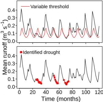
Fig. 4. Example of the variable threshold level method (TLM) to identify droughts for monthly runoff data. Based on the runoff
time series (black line), for each individual monthm, a threshold
Qthreshold(red line) is calculated (here taken as the 20th percentile).
Months with runoffQ≤Qthresholdare in a drought (red dots).
A graphical implementation of the variable TLM used to identify drought is presented in Fig. 4 for a time series of monthly runoff data. Since this data series shows consider-able seasonal variability, thresholds were defined for each month separately. Here, the 20th percentile for a given month (P20,T, whereT = 1, 2, ..., 12) was used as a threshold, which is given by the red line in Fig. 4 (top panel). During months for which the percentile value of runoff is below or similar to this threshold, a drought occurs. These months are identified by the red dots in Fig. 4 (bottom panel).
3.1.2 Consecutive dry period method
[image:5.595.52.286.63.300.2]The CDPM was implemented as follows:
1. Identify within the hydrological data series all time steps with a zero value.
2. For each of these identified time steps, calculate its con-secutive dry period numberNdry. Once a dry period is
followed by a positive value, the consecutive series is “broken”. The next time step containing a zero value af-ter such a wet period will then start again withNdry= 1.
3. Based on the series with consecutive dry period num-bers, the percentile statistics can be calculated (NP, whereP = 5, 10, 15, ..., 95 %). As such, based on the time series, it is possible to relate each consecutive pe-riod numberNdryto a given percentile statistic.
4. A drought is then identified using a given exceedance threshold, generally defined by a given percentile value
Nthreshold(e.g. 80th percentile). In case the consecutive
number of a given time step surpasses this threshold value (Ndry> Nthreshold), the region is assumed to
ex-perience a drought.
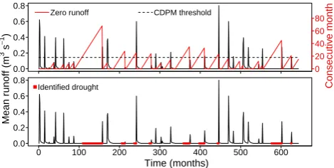
A hypothetical example for runoff data is presented in Fig. 5. For this time series, a considerable number of months with zero runoff is observed. For each of these months, the consecutive dry period numberNdry is calculated as given
by the red line in Fig. 5 (top panel). Months with a consec-utive dry period number larger than the defined percentile threshold (Ndry> Nthreshold) are in drought. The final result
of this procedure is presented in Fig. 5 (bottom panel), where months in drought are shown by the red dots.
3.2 Combining the characteristics of the TLM and CDPM
The previous sections presented the specific details behind the TLM and the CDPM to identify hydrological drought. In case each method is used separately, they either fail to iden-tify drought within drier environments (TLM) where runoff becomes zero, or are not applicable within temperate envi-ronments (CDPM) where runoff is always positive. However, by developing a procedure that is able to use the benefits of both techniques, a robust hydrological drought identification method can be obtained. This combined method was imple-mented according to the following procedure:
1. For each time series of a hydrological variable for each period of interest (e.g. day, month), a number of per-centile statistics are calculated (P= 5, 10, 15, ..., 95). 2. In case less than 5 percent of the time series contains a
value of zero (X5>0), the variable TLM is followed as
presented in Sect. 3.1.1. For situations where this does not hold, the variable TLM has to be combined with the CDPM.
0.0 0.2 0.4 0.6 0.8
0 20 40 60 80
Zero runoff CDPM threshold
Consecutiv
e month
0.0 0.2 0.4 0.6 0.8
0 100 200 300 400 500 600
Identified drought
Mean r
unoff (
m
3s
−
1)
[image:6.595.311.546.62.180.2]Time (months)
Fig. 5. Example of the consecutive dry period method (CDPM) to identify a hydrological drought for runoff data. Based on the monthly runoff data (black line), for months with zero runoff, its consecutive dry period number is calculated (red line). Based on the CDPM series, a given fixed exceedance threshold can be set (dashed line). Droughts are identified for those months that exhibit a CDPM value larger than the threshold (red dots).
3. For the time series withX5= 0, for each time step with
X= 0, its consecutive dry number Ndry is calculated,
from which again the different percentile statistics can be obtained (NP, whereP= 5, 10, 15, ..., 95). Notice that, contrary to the variable TLM implementation, the CDPM statistics are estimated as a fixed concept based on the entire time series for time steps with zero value observations without considering seasonality. This ap-proach was chosen, because, in areas with many short periods of zero runoff (e.g. every winter period during 2 to 3 months), a variable approach would give too many short droughts.
4. All positive data values (X >0) are then transformed into their corresponding percentile statistic. In case the calculated percentile value is smaller than or equal to the defined thresholdPT ,threshold (e.g. the 20th percentile),
a drought is assumed to occur.
5. Periods of positive runoff that experience a drought are combined with the zero runoff observations to obtain a new series. This series defines the consecutive number
Ndry,droughtfor all time steps, which are either zero or in
a drought.
6. Next, the corresponding percentile statistics are esti-mated for each time step with zero runoff. This is done by comparingNdry,droughtof the combined series
(step 5) to the statistics obtained from the consecutive zero runoff series only (step 3). If a time series has both zero and positive runoff in the given period of interest, both methods contribute to the transformation to per-centile statistics. It should be noted that the maximum percentile value for a zero runoff time step can never exceed the value 100−Fwet, whereFwetis the fraction
of interest. Therefore, the percentile fractions as calcu-lated according to the CDPM for dry periods are scaled. For example, if a monthly threshold is used, not every January in the entire time series has the same charac-teristics. In some years, runoff might be positive, while in other years a no-flow situation occurs. In this case, both the TLM and CDPM contribute to determining the percentile values. If runoff occurs in 60 % of the time series, percentiles derived from CDPM are rescaled to the lowest 40 (100−Fwet) percentiles. In other words,
the 50th percentile derived from the CDPM part of the method will become the 20th percentile for January. 7. The final result of this combined drought identification
procedure is a continuous series of estimated percentiles for both wet (high percentile values) and dry (low per-centiles values) conditions. All time steps that contain a percentile value below or equal to a defined thresh-oldPthreshold (here the 20th percentile) are assumed to
correspond to a drought.
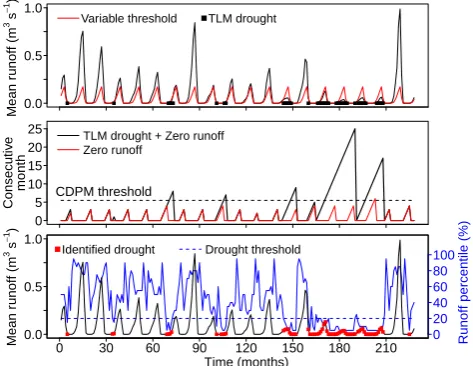
This procedure enables one to relate each time step to a given percentile value. By using the consecutive number of the combined series of zero or in a drought, the method tries to ensure that a hydrological drought observed for positive runoff data according to the variable TLM is generally fol-lowed by a drought according to the CDPM. A graphical example of the combined method to identify hydrological droughts is presented in Fig. 6 for part of a time series, which contains intermittent runoff data. Such a time series is gen-erally observed within a cold arid environment, where in the winter period as the result of below zero temperatures and the occurrence of snow, zero runoff values are observed. The first step is to calculate the variable threshold percentile (red line in Fig. 6, top panel). Next, for all periods with zero runoff, its consecutive dry number is estimated (red line in Fig. 6, middle panel), from which the CDPM drought threshold can be estimated (dashed line in Fig. 6, middle panel). A drought is observed for positive runoff values smaller than or equal to the variable threshold. These months in drought are then combined with the consecutive dry period series, to obtain a consecutive period series for which the observation is zero or in a drought (black line in Fig. 6, middle panel). Months for which the combined consecutive dry period is larger than the CDPM threshold are assumed to experience a drought as well. The final result of this procedure is presented in Fig. 6 (bottom panel), where each month defined to be in drought either with positive or zero runoff data is presented by the red dot. Figure 6 (bottom panel) also gives the correspond-ing runoff percentile statistic for each month.
0.0 0.5 1.0
TLM drought Variable threshold
Mean r
unoff (
m
3s
−
1)
0 5 10 15 20
25 TLM drought + Zero runoff
Zero runoff
Consecutiv
e
month CDPM threshold
0 20 40 60 80 100
Runoff percentile (%)
Identified drought Drought threshold
0.0 0.5 1.0
0 30 60 90 120 150 180 210
Mean r
unoff (
m
3s
−
1)
[image:7.595.309.546.64.247.2]Time (months)
Fig. 6. Combined drought identification method using characteris-tics of both the variable TLM (Fig. 4) and the fixed CDPM (Fig. 5). The runoff series in the upper panel (black line) contains multi-ple periods with zero runoff. Within the first step, monthly varying
runoff thresholdsQthreshold are calculated (red line). Months for
whichQ >0,Qthreshold>0 andQ≤Qthresholdare assumed to be
in a drought according to the TLM (black dots). For months with
Q= 0, the CDPM series (red line in middle panel) is used to obtain
a given CDPM fixed threshold (dashed line in middle panel). Next, the CDPM series is combined with TLM drought series to obtain the consecutive period of being either in a drought or zero (black line in middle panel). Based on this series, dry months that exceed the CDPM threshold are also assumed to be in a drought. Bottom panel presents the final result, with the months in a drought indicated as red dots.
4 Illustration of the generic drought identification method
4.1 Drought identification for observed discharge data
0
2
4
6
Maroni
1957 1958 1959 1960 1961 1962
0
40
80
Discharge percentile (%)
0
2
4
6
Q (
10
3m 3s
−
1)
Rhine
0
2
4
6
8
0
40
80
Discharge percentile (%)
1975 1976 1977 1978 1979 1980
0
2
4
6
8
Q (
10
3m 3s
−
1)
Observed discharge 20 percentile threshold
[image:8.595.50.284.62.335.2]Discharge percentile 20 percentile threshold
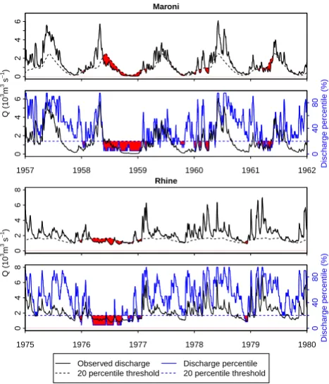
Fig. 7. Drought events (indicated in red) identified by the different methods for the Maroni and Rhine Rivers. Upper panel: TLM for Maroni River; second panel: combined method for Maroni River; third panel: TLM for Rhine River; fourth panel: combined method Rhine River. In all panels, the observed discharges are given (black line) and the threshold values (here the 20th percentile, dashed lines). From the observed discharge, percentile values for each day are calculated (blue line).
For the other two rivers, however, the situation is different. The Ellice and Ashburton Rivers have periods with zero dis-charge, which are caused by different processes (e.g. snow versus lack of precipitation; Sect. 2). For these two rivers, all three methods were applied to identify drought events. Re-sults of these drought analyses are shown in Figs. 8 and 9. In both rivers, the TLM determines drought events in the pe-riod when discharge is larger than zero and all pepe-riods with zero flow are classified as drought (Figs. 8 and 9). This is due to the methodology used here that drought occurs when discharge is lower or equal to the threshold. This leads to a relatively large number of drought events and a long average duration for the TLM (Table 2). When the CDPM is used, by definition no drought events are determined in the periods with discharge, so all drought events occur at the end of long zero flow periods. This leads to a relatively small number of droughts and shorter average durations than with the TLM.
By combining both methods, drought events both in the periods with runoff as well as in zero flow periods can be de-termined. This sometimes increases the duration of a drought event compared to the CDPM (Fig. 8), but also includes more shorter events compared to both methods separately.
0
0.1
0.2
Ashburton
0
100
200
300
Dr
y per
iods (d)
0
10
20
1988 1989 1990 1991 1992 1993
0
40
80
Discharge percentile (%)
0
10
20
Q (
m
3s
−
1)
Observed discharge 20 percentile threshold
Dry periods number 20 percentile threshold
[image:8.595.312.544.65.274.2]Discharge percentile 20 percentile threshold
Fig. 8. Drought events (indicated in red) identified by the differ-ent methods for the Ashburton River. The upper panel gives the TLM. Discharge values are shown as solid black line. The dashed line is the calculated threshold (20th percentile). Please note only the low flow values are given on y-axis. The middle panel gives drought events calculated with the CDPM. The consecutive dry pe-riods are indicated by the green line, and droughts are identified if periods exceed the threshold (dashed green line). When combining these methods, the discharge is converted to percentile values (low-est panel, blue solid line). If the percentile value drops below or equals the 20 % (dashed blue) line, the month is in drought.
Table 2. Drought characteristics for the different rivers identified with the drought analysis methods.
River Period Method Number of
Duration (days) droughts avg min max
Rhine 1950–2007 combined 242 17.4 1 137
Maroni 1952–1995 combined 170 13.8 1 145
Ashburton 1973–2005 TLM 69 75.9 1 304
CDPM 19 53.6 11 184
combined 51 51.5 1 304
Ellice 1971–1996 TLM 55 90.7 1 231
CDPM 23 37.3 6 74
combined 61 27.0 1 93
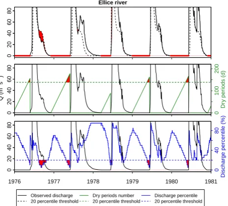
[image:8.595.309.548.455.564.2]Ellice river
0
40
80
20
60
0
100
200
Dr
y per
iods (d)
0
40
80
20
60
1976 1977 1978 1979 1980 1981
0
40
80
Discharge percentile (%)
0
40
80
20
60
Q (
m
3s
−
1)
Observed discharge 20 percentile threshold
Dry periods number 20 percentile threshold
[image:9.595.327.526.62.242.2]Discharge percentile 20 percentile threshold
Fig. 9. Drought events (indicated in red) identified by the differ-ent methods for the Ellice River. The upper panel gives the TLM. Discharge values are shown as solid black line. The dashed line is the calculated threshold (20th percentile). The middle panel gives drought events calculated with the CDPM; the consecutive dry pe-riods are indicated by the green line, and droughts are identified if periods exceed the threshold (dashed green line). When combining these methods, the discharge is converted to percentile values (low-est panel, blue solid line). If the percentile value drops below or equals the 20 % (dashed blue) line, the month is in drought.
also the shortest maximum drought duration. For the Ash-burton River, the maximum durations determined with the TLM and with the combined method are the same. This is a drought event that already started before a zero discharge period, which caused the entire zero discharge period to be determined as drought by both methods. For the Ellice River, there is a large difference in maximum durations for the TLM and combined method. This implies that the largest drought of the TLM was a zero runoff period only, without preced-ing drought days. Such drought events will be shorter or ex-cluded in the combined method, because they are determined with the CDPM part of the method.
More examples of the drought analyses with observed dis-charge data are given in Appendix A.
4.2 Drought identification for simulated global runoff data
Besides on river basin scale observations, the drought analy-sis methods were also tested at the global scale using the en-semble median results of five different LSMs. At the global scale, the TLM identifies drought events in all continents, while the CDPM only gives results in cells where zero runoff periods occur. These cells are shown in Fig. 11. A small part of the world is simulated without runoff during the
1 2 5 10 20 50 100 200
0
20
40
60
80
100
Duration (days)
Occurrence [%]
TLM Ashburton CDPM Ashburton Combined method Ashburton TLM Ellice
[image:9.595.53.286.64.274.2]CDPM Ellice Combined method Ellice
Fig. 10. Cumulative distribution of the duration of drought events determined with all three methods for Ellice River (red) and Ash-burton River (black). Dashed lines give the drought durations de-termined with the TLM. Dotted lines show the durations from the CDPM, and the solid lines are durations calculated with the com-bined method.
entire time series. These cells were excluded from all anal-yses (black area in Fig. 11). The CDPM mainly determines drought events in Africa and Australia, since the other con-tinents have no or only a small area of cells with zero runoff periods. Therefore, to compare the three methods, results of the continents Africa, Australia and, to illustrate regions with continuous runoff, Europe are given (Fig. 12).
According to the TLM, a large fraction of Africa was in drought from 1982 until 2001. This is due to the em-ployed methodology, which classifies all zero runoff periods as drought events, and thus gives a large area in drought in Africa. The CDPM only shows a small fraction of Africa in drought, since it is only relevant for part of the conti-nent. However, both methods identify the 1980s as dry years, which correspond with literature (Dai et al., 2004; Sheffield et al., 2009), and show an increase in drought in the 1980s and 1990s as compared to the 1960s and 1970s. By com-bining the methods, the erroneous droughts identified by the TLM due to the recurring zero runoff periods, and the lack of droughts in regions with runoff when using the CDPM, can be avoided. Therefore, the combined method gives a much smaller area in drought in Africa than the TLM, but larger than the CDPM. The historic drought years in the 1980s are still reflected, and trends seem to be similar for all methods.
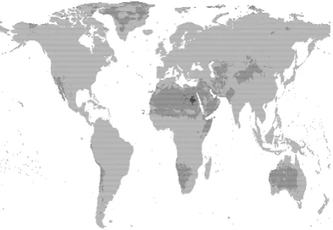
Fig. 11. Location of the grid cells (dark gray colour) in which peri-ods with zero runoff occur according to the ensemble median of five LSMs and where the CDPM can be applied. The black cells indi-cate the area without runoff during the entire time series (hyper-arid cells), which have been excluded from the analysis.
combined method, which shows higher fractions in drought in this period.
The results of the drought analyses with all three meth-ods for Europe are given to illustrate the method in a climate without zero runoff periods. Obviously, in such a climate, the CDPM does not give any drought, which means that the com-bined method gives the same results as the TLM. This is also visible in Fig. 12. The largest fraction in drought is identi-fied in 1975–1976, which is a well-known drought event in Europe (Stahl, 2001; Zaidman et al., 2002).
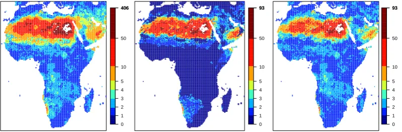
For each grid cell, drought characteristics, such as the number of droughts and drought duration, can be calculated from the time series with drought events. Figure 13 shows the average duration of droughts (in months) determined with all three methods for each grid cell in Africa. Africa is chosen as illustration, because a relatively large area of the conti-nent consists of drier regions and the differences between the methods are thus expected to be largest here. The maximum average drought duration differs substantially between the TLM and combined method. The area with a long average drought duration is largest with the TLM and smallest with the combined method.
5 Discussion
The newly developed method is suitable for global studies, which have to cope with drought analysis of regions with a wide variety of flow types in a single analysis, i.e. peren-nial, intermittent and ephemeral flow. The method allows characterization of drought events that continue from peri-ods with runoff into periperi-ods without runoff and vice versa. This means the method especially shows its relevance for the transitional areas, because beyond these regions, results are identical to the widely applied threshold level method, or
2 4 6 8 10
12 Africa
2 4 6 8 10 12
1965 1980 1995
2 4 6 8 10 12
Australia
1965 1980 1995
Europe
1965 1980 1995
Year
Month
0 12 24 36 48 60
Fraction in drought (%)
Fig. 12. Fraction in drought (%) of the area for 3 continents (Africa, Australia and Europe) as identified with the different methods from the ensemble median of 5 LSMs. Top row: TLM; middle row: CDPM; bottom row: combined method.
hydrological analysis is meaningless because flow is negligi-ble. Since these areas are expected to increase in the future (Romm, 2011), this method can be a valuable addition to ex-isting drought identification tools.
The new method uses one uniform threshold level for the TLM across the world, which overcomes the selection of dif-ferent percentiles in difdif-ferent climates, which makes a global comparison difficult. For example, Fleig et al. (2006) used in their global study of drought in streamflow very high thresh-old values, e.g.Q50–Q80 for intermittent streams, to avoid
threshold values of zero, whereas for perennial rivers sub-stantially lower thresholds were applied. Hisdal et al. (2004) recommend thresholds between Q30 and Q5 for the latter
category of rivers. Periods with a zero threshold are still excluded in the studies using only TLM. In this study, we have used one uniform threshold for the variable TLM, the 20th percentile value. The new method is flexible, and other threshold levels can be chosen depending on the purpose of the analysis.
[image:10.595.50.286.63.226.2]0 1 2 3 4 5 10 50 406
406
0 1 2 3 4 5 10 50 93
93
0 1 2 3 4 5 10 50 93
[image:11.595.100.500.63.194.2]93
Fig. 13. Average durations of droughts in months for each grid cell in Africa as identified with all three methods from the ensemble median of 5 LSMs. Left panel: TLM; middle panel: CDPM; right panel: combined method.
zero runoff periods are completely classified as droughts. Other studies, e.g. Tallaksen et al. (2009), only classify a pe-riod as in drought when the runoff is below the threshold. In this case, the TLM would underestimate the number and du-ration of drought events compared to the new method, since periods with zero runoff are never considered as a drought when theQ20 is equal to zero (or very high threshold levels
are needed). So regardless of the choice for a certain method-ology in the TLM, the combined method will lead to more re-alistic results by including both the periods with and without runoff.
By including all periods, the combined method considers the entire time series, leading to more minor drought events. To reduce this number, pooling of droughts can be done in the same way as after the traditional threshold level method (Tallaksen et al., 1997; Fleig et al., 2006). Several metrics can be used to make a selection from the identified drought events, e.g. based on duration or severity. However, due to zero runoff periods, not all drought characteristics can always be identified. For example, the deficit volume simply cannot be determined from the periods with zero runoff, whereas in other periods this is possible. Depending on the purpose of a drought analysis study, spatial coverage of droughts can be investigated using a cluster algorithm (Andreadis et al., 2005; Corzo Perez et al., 2011) after the identification of droughts with the combined method.
In the current paper, we used the ensemble median of five LSMs to illustrate the new method. Haddeland et al. (2011) found in their multi-model analysis, which included 11 dif-ferent large-scale models (both GHMs and LSMs), that in general the models overestimate runoff in semi-arid and arid basins. They also found a very large spread in runoff between the models in these areas. The LSMs gave lower runoff val-ues than the GHMs and were closer to observations (Hadde-land et al., 2011), which was the reason to use LSMs only in this study. Global or continental hydrological analyses ex-tensively use output of large-scale models (e.g. Andreadis et al., 2005; Dirmeyer et al., 2006; Sheffield et al., 2009; Corzo Perez et al., 2011; Haddeland et al., 2011; Prudhomme
et al., 2011; Stahl et al., 2011, 2012). As large-scale mod-els have difficulties capturing all hydrological processes, in-finitesimal runoff values that may occur in model results can be set to zero using a minimum threshold, depending on the purpose of the study. The number of grid cells that experi-ence zero runoff periods can be different for each individual model. Some models tend to have very long recession pe-riods, leading to extremely small, but non-zero runoff. For example, in the ET-climate, the ensemble median now has runoff almost everywhere, while in observations of the El-lice River long zero runoff periods occur. When these periods with small values are considered to be zero runoff periods, the area, in which the combined method is beneficial, will substantially increase.
Since in this study model results are only used as illus-tration of the method, they have not been validated against observations. Further drought analyses with large-scale mod-els will require additional validation, in which limitations in measuring very low flows (e.g. Rees et al., 2004) should be taken into account.
6 Conclusions
A B C D E
● ●
●
Mekong Humboldt
[image:12.595.310.546.62.241.2]Fortescue
Fig. A1. Locations of the discharge gauges of the additional rivers within the 5 major climate types.
1. The new hydrological drought identification method is well able to define drought across the globe in a consis-tent manner.
2. Compared to the classical variable threshold level method, the new combined method is much better able to define drought in the transition areas of the world – from the hot and dry (hyper-arid) to the wetter cli-mates (semi-arid) or from the extremely cold (polar frost) to the warmer climates (polar tundra). The thresh-old level method either overestimates the drought events in these regions by identifying all zero runoff periods as droughts, or underestimates them by excluding these periods.
3. The combined method can be applied to both areas with and without runoff, whereas the CDPM is only applica-ble in areas with zero runoff and thus in a limited part of the world.
Overall, the combination of the TLM and the CDPM leads to a more robust drought identification method. As such, the combined method is able to identify drought within different climate regions, which enables one to perform global drought analysis in a consistent, more reliable manner. In a follow-up paper, we will implement this method at global scale for runoff data as simulated by 10 different global hydrological and land surface models.
Appendix A
Extended drought analysis on observed discharge data
Observed daily discharge data of four rivers, which pro-vide a wide range of runoff regimes, were used to illus-trate the new method for hydrological drought identification (Sect. 4.1). This dataset is extended in this section with three extra selected rivers, with different regimes and in differ-ent climates, to further test robustness of the newly devel-oped drought identification method under different climate
0
20000
40000
Mekong
regime[, 2]
Humboldt
0
20
40
Fortescue
J F M A M J J A S O N D
0
40
80
Q (
m
3s
−
[image:12.595.48.287.64.190.2]1)
Fig. A2. Yearly regimes of the additional rivers based on average daily discharge (black line) and the spread between the 10th and 90th percentile values (gray zone).
0
20
40
10
30
Mekong
1988 1989 1990 1991 1992 1993
0
40
80
Discharge percentile (%)
0
20
40
10
30
Q (
10
3m 3s
−
1)
Humboldt
0
20
40
0
40
80
Discharge percentile (%)
1991 1992 1993 1994 1995 1996
0
20
40
Q (
m
3s
−
1)
Observed discharge 20 percentile threshold
Discharge percentile 20 percentile threshold
[image:12.595.310.545.301.572.2]Table A1. Drought characteristics for the additional rivers identified with the drought analysis methods.
River Period Method Number of
Duration (days) droughts avg min max
Mekong 1968–1993 combined 128 12.7 1 150
Humboldt 1946–2008 combined 196 23.5 1 340
Fortescue 1969–1999 TLM 76 39.6 1 315
CDPM 7 50.7 16 115
combined 69 35.1 1 315
[image:13.595.49.290.93.175.2]conditions. The three rivers discussed in this section are the Fortescue (Australia), Mekong (Asia) and Humboldt (North America) Rivers. Discharge data from these rivers were made available by the Global Runoff Data Centre (GRDC, 2011). Figure A1 gives the approximate locations of the discharge gauges of these rivers in the different climates. For all three rivers, their mean daily discharge regimes, as well as the spread between the 10th and 90th percentile values, are shown in Fig. A2. The Fortescue River is an intermittent river; the Mekong and Humboldt Rivers are classified as perennial rivers.
The same drought analysis methods (Sect. 3) have been used for these three rivers as for the other analyses: TLM, CDPM and combined method. Figure A3 and Table A1 give the results of the drought analyses for the Humboldt and Mekong Rivers. For these perennial rivers, the CDPM does not yield additional information. As was expected, results were the same for both the TLM and the combined method.
Results of the different drought analysis methods for the Fortescue River are given in Fig. A4 and Table A1. The TLM method identifies all periods with zero runoff as droughts due to the definition used here. This leads to relatively long du-rations. The CDPM has identified only seven drought events, which leads to a very long average duration compared to the other methods. Since the combined method includes the events in periods with and without runoff, more short events are identified compared to the CDPM and the long events caused by zero runoff in the TLM are excluded. This leads to a shorter average duration with the combined method. The drought event with the maximum duration in this discharge series is a drought that started in a period with runoff and continued into a period without runoff. Both the TLM and combined method therefore gave a maximum duration of 315 days (Table A1). Results for the additional rivers pre-sented in this Appendix correspond with the results found in observed discharge data from the four rivers in Sect. 4.1.
Fortescue
0
0.5
1
1.5
2
0
100
200
Dr
y per
iods (d)
0
0.5
1
1.5
2
1983 1984 1985 1986 1987 1988
0
40
80
Discharge percentile (%)
0
0.5
1
1.5
2
Q (
m
3s
−
1)
Observed discharge 20 percentile threshold
Dry periods number 20 percentile threshold
Discharge percentile 20 percentile threshold
Fig. A4. Drought events (indicated in red) identified by the different methods for the Fortescue River. The upper panel gives the TLM. Discharge values are shown as solid black line; the dashed line is the calculated threshold (20th percentile). The middle panel gives drought events calculated with the CDPM. The consecutive dry pe-riods are indicated by the green line, and droughts are identified if periods exceed the threshold (dashed green line). When combining these methods, the discharge is converted to percentile values (low-est panel, blue solid line). If the percentile value drops below or equals the 20 % (dashed blue) line, the month is in drought.
Acknowledgements. The authors wish to acknowledge all
mod-ellers for supplying the results of the LSMs: Natalie Bertrand (Orchidee), Douglas Clark (JULES), Sandra Gomes (HTESSEL), Naota Hanasaki (H08) and Sujan Koirala (MATSIRO). The authors also want to thank the Global Runoff Data Centre (56068 Koblenz, Germany) for providing the observed discharge data. Furthermore, the authors thank Graham Weedon (UK MetOffice) for supplying the WATCH forcing data. This research has been financially supported by the EU-FP6 Project WATCH (contract 036946), the EU-FP7 Project IMPRINTS (FP7-ENV-2008-1-226555) and the EU-FP7 Project DROUGHT-R&SPI (contract 282769). This research is part of the programme of the Wageningen Institute for Environment and Climate Research (WIMEK-SENSE) and it supports the work of the EURO-FRIEND programme.
References
Andreadis, K. M., Clark, E. A., Wood, A. W., Hamlet, A. F., and Lettenmaier, D. P.: Twentieth-century drought in the contermi-nous United States, J. Hydrometeorol., 6, 985–1001, 2005. Anyah, R. O., Weaver, C. P., Miguez-Macho, G., Fan, Y., and
Robock, A.: Incorporating water table dynamics in climate mod-eling: 3. Simulated groundwater influence on coupled land-atmosphere variability, J. Geophys. Res.-Atmos., 113, D07103, doi:10.1029/2007JD009087, 2008.
Balsamo, G., Viterbo, P., Beljaars, A., van den Hurk, B., Hirschi, M., Betts, A. K., and Scipal, K.: A Revised Hydrology for the ECMWF Model: Verification from Field Site to Terrestrial Wa-ter Storage and Impact in the Integrated Forecast System, J. Hy-drometeorol., 10, 623–643, 2009.
Best, M. J., Pryor, M., Clark, D. B., Rooney, G. G., Essery, R .L. H., M´enard, C. B., Edwards, J. M., Hendry, M. A., Porson, A., Gedney, N., Mercado, L. M., Sitch, S., Blyth, E., Boucher, O., Cox, P. M., Grimmond, C. S. B., and Harding, R. J.: The Joint UK Land Environment Simulator (JULES), model description – Part 1: Energy and water fluxes, Geosci. Model Dev., 4, 677–699, doi:10.5194/gmd-4-677-2011, 2011.
BoM: Living with Drought, available at: http://www.bom.gov.au/ climate/drought/livedrought.shtml, last access: July 2011, Aus-tralian Bureau of Meteorology, 1997.
Clark, D. B., Mercado, L. M., Sitch, S., Jones, C. D., Gedney, N., Best, M. J., Pryor, M., Rooney, G. G., Essery, R. L. H., Blyth, E., Boucher, O., Harding, R. J., Huntingford, C., and Cox, P. M.: The Joint UK Land Environment Simulator (JULES), model descrip-tion – Part 2: Carbon fluxes and vegetadescrip-tion dynamics, Geosci. Model Dev., 4, 701–722, doi:10.5194/gmd-4-701-2011, 2011. Corzo Perez, G. A., van Huijgevoort, M. H. J., Voß, F., and van
Lanen, H. A. J.: On the spatio-temporal analysis of hydrological droughts from global hydrological models, Hydrol. Earth Syst. Sci., 15, 2963–2978, doi:10.5194/hess-15-2963-2011, 2011. Dai, A.: Drought under global warming: a review, WIREs-Climate
Change, 2, 45–65, 2011.
Dai, A., Trenberth, K. E., and Qian, T. T.: A global dataset of Palmer Drought Severity Index for 1870–2002: Relationship with soil moisture and effects of surface warming, J. Hydrometeorol., 5, 1117–1130, 2004.
de Rosnay, P. and Polcher, J.: Modelling root water uptake in a com-plex land surface scheme coupled to a GCM, Hydrol. Earth Syst. Sci., 2, 239–255, doi:10.5194/hess-2-239-1998, 1998.
Deni, S. M. and Jemain, A. A.: Mixed log series geometric dis-tribution for sequences of dry days, Atmos. Res., 92, 236–243, doi:10.1016/j.atmosres.2008.10.032, 2009.
Dirmeyer, P. A., Gao, X., Zhao, M., Guo, Z., Oki, T., and Hanasaki, N.: GSWP-2 – Multimodel analysis and implications for our per-ception of the land surface, B. Am. Meteorol. Soc., 87, 1381– 1397, doi:10.1175/BAMS-87-10-1381, 2006.
Dracup, J. A., Lee, K. S., and Paulson, E. G.: On the Definition of Droughts, Water Resour. Res., 16, 297–302, 1980.
European Commission: Communication Addressing the chal-lenge of water scarcity and droughts in the European Union, COM2007 414, European Commission, DG Environment, Brus-sels, 2007.
Fleig, A. K., Tallaksen, L. M., Hisdal, H., and Demuth, S.: A global evaluation of streamflow drought characteristics, Hydrol. Earth Syst. Sci., 10, 535–552, doi:10.5194/hess-10-535-2006, 2006.
Gao, X. and Dirmeyer, P. A.: A multimodel analysis, validation, and transferability study of global soil wetness products, J. Hydrom-eteorol., 7, 1218–1236, doi:10.1175/JHM551.1, 2006.
GRDC: Global Runoff Data Centre, available at: http://www.bafg. de/GRDC, 56068 Koblenz, Germany, 2011.
Griffiths, M. L. and Bradley, R. S.: Variations of twentieth-century temperature and precipitation extreme indicators in the northeast United States, J. Climate, 20, 5401–5417, doi:10.1175/2007JCLI1594.1, 2007.
Groisman, P. Y. and Knight, R. W.: Prolonged dry episodes over the conterminous United States: New tendencies emerg-ing duremerg-ing the last 40 years, J. Climate, 21, 1850–1862, doi:10.1175/2007JCLI2013.1, 2008.
Guo, Z., Dirmeyer, P. A., Gao, X., and Zhao, M.: Improving the quality of simulated soil moisture with a multi-model en-semble approach, Q. J. Roy. Meteorol. Soc., 133, 731–747, doi:10.1002/qj.48, 2007.
Haddeland, I., Clark, D. B., Franssen, W., Ludwig, F., Voss, F., Arnell, N. W., Bertrand, N., Best, M., Folwell, S., Gerten, D., Gomes, S., Gosling, S. N., Hagemann, S., Hanasaki, N., Harding, R., Heinke, J., Kabat, P., Koirala, S., Oki, T., Polcher, J., Stacke, T., Viterbo, P., Weedon, G. P., and Yeh, P.: Multi-Model Estimate of the Global Terrestrial Water Balance: Setup and First Results, J. Hydrometeorol., 12, 869–884, doi:10.1175/2011JHM1324.1, 2011.
Hanasaki, N., Kanae, S., Oki, T., Masuda, K., Motoya, K., Shi-rakawa, N., Shen, Y., and Tanaka, K.: An integrated model for the assessment of global water resources – Part 1: Model descrip-tion and input meteorological forcing, Hydrol. Earth Syst. Sci., 12, 1007–1025, doi:10.5194/hess-12-1007-2008, 2008. Hisdal, H., Tallaksen, L. M., Clausen, B., Peters, E., and
Gus-tard, A.: Hydrological Drought Characteristics, in: Hydrological Drought Processes and Estimation Methods for Streamflow and Groundwater, edited by: Tallaksen, L. M. and van Lanen, H. A. J., Elsevier Science B. V., Developments in Water Science, 48, 139–198, 2004.
Im, E. S., Jung, I. W., and Bae, D. H.: The temporal and spatial structures of recent and future trends in extreme indices over Ko-rea from a regional climate projection, Int. J. Climatol., 31, 72– 86, doi:10.1002/joc.2063, 2011.
Jaranilla-Sanchez, P. A., Wang, L., and Koike, T.: Modeling the hydrologic responses of the Pampanga River basin, Philippines: A quantitative approach for identifying droughts, Water Resour. Res., 47, W03514, doi:10.1029/2010WR009702, 2011. Kallis, G.: Droughts, Ann. Rev. Environ. Resour., 33, 85–118,
doi:10.1146/annurev.environ.33.081307.123117, 2008. Kampragou, E., Apostolaki, S., Manoli, E., Froebrich, J., and
As-simacopoulos, D.: Towards the harmonization of water-related policies for managing drought risks across the EU, Environ. Sci. Policy, 14, 815–824, doi:10.1016/j.envsci.2011.04.001, 2011. Koirala, S.: Explicit representation of groundwater process in a
global-scale land surface model to improve hydrological predic-tions, Ph.D. thesis, The University of Tokyo, 2010.
Koster, R. D. and Suarez, M. J.: Soil moisture memory in cli-mate models, J. Hydrometeorol., 2, 558–570,
doi:10.1175/1525-7541(2001)002<0558:SMMICM>2.0.CO;2, 2001.
D., Oki, T., Oleson, K., Pitman, A., Sud, Y. C., Taylor, C. M., Verseghy, D., Vasic, R., Xue, Y. K., Yamada, T., and Team, G.: Regions of strong coupling between soil moisture and precipi-tation, Science, 305, 1138–1140, doi:10.1126/science.1100217, 2004.
McKee, T., Doesken, N., and Kleist, J.: The relationship of drought frequency and duration to time scales, in: Preprints, Eight Con-ference on Applied Climatology, 17–22 January, Anaheim, Cali-fornia, 179–184, 1993.
Mishra, A. K. and Singh, V. P.: A review of drought concepts, J. Hy-drol., 391, 202–216, doi:10.1016/j.jhydrol.2010.07.012, 2010. Peel, M. C., Finlayson, B. L., and McMahon, T. A.: Updated
world map of the K¨oppen-Geiger climate classification, Hy-drol. Earth Syst. Sci., 11, 1633–1644, doi:10.5194/hess-11-1633-2007, 2007.
Prudhomme, C., Parry, S., Hannaford, J., Clark, D. B., Hagemann, S., and Voss, F.: How well do large-scale models reproduce re-gional hydrological extremes in Europe?, J. Hydrometeorol., 12, 1181–1204, doi:10.1175/2011JHM1387.1, 2011.
Rees, G., Marsh, T. J., Roald, L., Demuth, S., van Lanen, H. A. J., and Kaˇsp´arek, L.: Hydrological Data, in: Hydrological Drought Processes and Estimation Methods for Streamflow and Ground-water, edited by: Tallaksen, L. M. and van Lanen, H. A. J., Else-vier Science B. V., Developments in Water Science, 48, 99–138, 2004.
Romm, J.: The next dust bowl, Nature, 478, 450–451, 2011. Seneviratne, S. I., Nicholls, N., Easterling, D., Goodess, C. M.,
Kanae, S., Kossin, J., Luo, Y., Marengo, J., McInnes, K., Rahimi, M., Reichstein, M., Sorteberg, A., Vera, C., and Zhang, X.: Changes in climate extremes and their impacts on the natural physical environment, in: Managing the Risks of Extreme Events and Disasters to Advance Climate Change Adaptation, edited by: Field, C. B., Barros, V., Stocker, T. F., Qin, D., Dokken, D. J., Ebi, K. L., Mastrandrea, M. D., Mach, K. J., Plattner, G. K., Allen, S. K., Tignor, M., and Midgley, P. M., A Special Report of Working Groups I and II of the Intergovernmental Panel on Cli-mate Change (IPCC), Cambridge University Press, Cambridge, UK, and New York, NY, USA, 109–230, 2012.
Sheffield, J. and Wood, E. F.: Characteristics of global and regional drought, 1950–2000: Analysis of soil moisture data from off-line simulation of the terrestrial hydrologic cycle, J. Geophys. Res.-Atmos., 112, D17115, doi:10.1029/2006JD008288, 2007. Sheffield, J., Andreadis, K. M., Wood, E. F., and Lettenmaier, D. P.:
Global and Continental Drought in the Second Half of the Twen-tieth Century: Severity-Area-Duration Analysis and Temporal Variability of Large-Scale Events, J. Climate, 22, 1962–1981, 2009.
Stahl, K.: Hydrological Drought – a Study across Europe, Ph.D. the-sis, available at: http://www.freidok.uni-freiburg.de/volltexte/ 202/, Albert-Ludwigs-Universit¨at Freiburg, Freiburg, Germany, 2001.
Stahl, K., Tallaksen, L. M., Gudmundsson, L., and Christensen, J. H.: Streamflow Data from Small Basins: A Challenging Test to High-Resolution Regional Climate Modeling, J. Hydrometeo-rol., 12, 900–912, doi:10.1175/2011JHM1356.1, 2011.
Stahl, K., Tallaksen, L. M., Hannaford, J., and van Lanen, H. A. J.: Filling the white space on maps of European runoff trends: estimates from a multi-model ensemble, Hydrol. Earth Syst. Sci., 16, 2035–2047, doi:10.5194/hess-16-2035-2012, 2012. Takata, K., Emori, S., and Watanabe, T.: Development of
the minimal advanced treatments of surface interaction and runoff, Global Planet. Change, 38, 209–222, doi:10.1016/S0921-8181(03)00030-4, 2003.
Tallaksen, L. M. and van Lanen, H. A. J. (Eds.): Hydrological drought: processes and estimation methods for streamflow and groundwater, Elsevier Science BV, Developments in Water Sci-ence, 48, The Netherlands, 2004.
Tallaksen, L. M., Madsen, H., and Clausen, B.: On the definition and modelling of streamflow drought duration and deficit vol-ume, Hydrolog. Sci. J., 42, 15–33, 1997.
Tallaksen, L. M., Hisdal, H., and van Lanen, H. A. J.: Space-time modelling of catchment scale drought characteristics, J. Hydrol., 375, 363–372, 2009.
Tallaksen, L. M., Stahl, K., and Wong, G.: Space-time characteris-tics of large-scale droughts in Europe derived from streamflow observations and WATCH multi-model simulations, WATCH Technical Report 48, available at: http://www.eu-watch.org/ publications/technical-reports (last access: 31 July 2012), 2011. Van Lanen, H. A. J. and Tallaksen, L. M.: Drought in Europe, in:
Proc. Water Down Under 2008, edited by: Lambert, M., Daniell, T., and Leonard, M., Adelaide, Australia, 14–17 April 2008, 98– 108, 2008.
Vincent, L. A. and Mekis, E.: Changes in daily and extreme temper-ature and precipitation indices for Canada over the twentieth cen-tury, Atmos. Ocean, 44, 177–193, doi:10.3137/ao.440205, 2006. Wanders, N., van Lanen, H. A. J., and van Loon, A. F.: Indicators for drought characterization on a global scale, WATCH Technical Report 24, available at: http://www.eu-watch.org/publications/ technical-reports (last access: 31 July 2012), 2010.
Weedon, G. P., Gomes, S., Viterbo, P., Shuttleworth, W. J., Blyth,
E., ¨Osterle, H., Adam, J. C., Bellouin, N., Boucher, O., and Best,
M.: Creation of the WATCH Forcing Data and its use to as-sess global and regional reference crop evaporation over land during the twentieth century, J. Hydrometeorol., 12, 823–848, doi:10.1175/2011JHM1369.1, 2011.
Wetherald, R. T. and Manabe, S.: Simulation of hydrologic changes associated with global warming, J. Geophys. Res.-Atmos., 107, 4379, doi:10.1029/2001JD001195, 2002.
Wilhite, D. A. (Ed.): DROUGHT A Global Assesment, Vol. I & II, Routledge Hazards and Disasters Series, Routledge, London, 2000.
Yevjevich, V.: An objective approach to definition and investiga-tions of continental hydrologic droughts, Hydrology papers 23, Colorado State University, Fort Collins, USA, 1967.