Parameter optimisation for a better representation of drought by LSMs: inverse modelling vs sequential data assimilation

https://doi.org/10.5194/hess-21-4861-2017 © Author(s) 2017. This work is distributed under the Creative Commons Attribution 3.0 License.

Parameter optimisation for a better representation of drought by

LSMs: inverse modelling vs. sequential data assimilation

Hélène Dewaele, Simon Munier, Clément Albergel, Carole Planque, Nabil Laanaia, Dominique Carrer, and Jean-Christophe Calvet

CNRM – UMR3589 (Météo-France, CNRS), Toulouse, 31057, France

Correspondence to:Jean-Christophe Calvet ([email protected]) Received: 2 March 2017 – Discussion started: 17 March 2017

Revised: 16 August 2017 – Accepted: 18 August 2017 – Published: 28 September 2017

Abstract. Soil maximum available water content (Max-AWC) is a key parameter in land surface models (LSMs). However, being difficult to measure, this parameter is usu-ally uncertain. This study assesses the feasibility of using a 15-year (1999–2013) time series of satellite-derived low-resolution observations of leaf area index (LAI) to estimate MaxAWC for rainfed croplands over France. LAI interannual variability is simulated using the CO2-responsive version of the Interactions between Soil, Biosphere and Atmosphere (ISBA) LSM for various values of MaxAWC. Optimal value is then selected by using (1) a simple inverse modelling tech-nique, comparing simulated and observed LAI and (2) a more complex method consisting in integrating observed LAI in ISBA through a land data assimilation system (LDAS) and minimising LAI analysis increments. The evaluation of the MaxAWC estimates from both methods is done using sim-ulated annual maximum above-ground biomass (Bag) and straw cereal grain yield (GY) values from the Agreste French agricultural statistics portal, for 45 administrative units pre-senting a high proportion of straw cereals. Significant cor-relations (p value<0.01) between Bag and GY are found for up to 36 and 53 % of the administrative units for the in-verse modelling and LDAS tuning methods, respectively. It is found that the LDAS tuning experiment gives more real-istic values of MaxAWC and maximumBagthan the inverse modelling experiment. Using undisaggregated LAI observa-tions leads to an underestimation of MaxAWC and maximum Bagin both experiments. Median annual maximum values of disaggregated LAI observations are found to correlate very well with MaxAWC.

1 Introduction

Extreme weather conditions markedly affect agricultural pro-duction. The interannual variability of rainfed crop yields is driven to a large extent by the climate variability. Compar-ing agricultural statistics to climate data shows the impact of atmospheric conditions on vegetation production. For exam-ple, lower temperature in northern Europe tends to shorten the period of crop growth. Conversely, persistent high tem-peratures as well as droughts in southern Europe are linked to negative anomalies of crop yields (Olesen et al., 2011). Li et al. (2010) showed that air temperature tends to influence mean crop yields at small scales (400 to 600 km), whereas rainfall drives crop yields at larger scales (50 to 300 km). Capa-Morocho et al. (2014) also showed the influence of air temperature on crop yields. They established a link between temperature anomalies related to the El Niño phenomenon and potential crop yield anomalies, obtained from reanalysis data and crop model, respectively.

transpi-ration along the vegetation growing cycle (Portoghese et al., 2008; Piedallu et al., 2011). MaxAWC is constrained by soil parameters and by the plant rooting depth. In regions vulner-able to drought risk exposure, MaxAWC is a key driver of the plant response to the climate variability.

Soil characteristics influence the vegetation response to climate (Folberth et al., 2016). In a model benchmark-ing study (Eitzbenchmark-inger et al., 2004) simulated evapotranspi-ration, soil moisture and biomass were compared with ob-servations. Eitzinger et al. used three crop models that dif-fer in the representation of the available soil water content (AWC): WOFOST (WOrld Food Studies model; Van Diepen et al., 1989), CERES (Crop Environment REsource Synthe-sis model; Ritchie and Otter, 1985) and SWAP (Statewide Agricultural Production model; van Dam et al., 1997). They showed that a better description of rooting depth and evapo-transpiration, taking account of soil type and crop type, could significantly improve these models. Tanaka et al. (2004), Por-toghese et al. (2008) and Piedallu et al. (2011) have high-lighted the important role of the soil characteristics (soil tex-ture, rooting depth) on MaxAWC. Soylu et al. (2011) and Wang et al. (2012) illustrated the major impact of Max-AWC on evapotranspiration. While soil properties such as soil texture determine the soil water holding capacity (in kg m−3), information on rooting depth is needed to deter-mine MaxAWC (in kg m−2). A better representation of Max-AWC could improve the simulated interannual variability of both water fluxes and vegetation biomass by LSMs.

The lack of in situ observations of MaxAWC to calibrate and assess LSMs limits the ability of LSMs to represent drought effects on plants. Using satellite observations and data assimilation techniques could be a solution to this prob-lem. A list of atmospheric, oceanic and terrestrial essential climate variables (ECVs) which can be monitored at a global scale from remote sensing observations was proposed by the Global Climate Observing System (GCOS). Leaf area index (LAI), fraction of absorbed photosynthetically active radia-tion (FAPAR) and soil moisture are key ECVs for land sur-face modelling. The use of these satellite-derived products to verify LSM simulations or to optimise key LSM parame-ters has been assessed by several authors (e.g. Becker-Reshef et al., 2010; Crow et al., 2012; Ferrant et al., 2014; Ford et al., 2014; Ghilain et al., 2012; Ichii et al., 2009; Kowalik et al., 2014; Szczypta et al., 2012, 2014). Data assimilation is a field of active research. Data assimilation techniques al-low the integration of different observation types (e.g. in situ or satellite derived) into LSMs in order to optimally combine them with model outputs: the correction applied to the model state is called the increment and the corrected model state is the analysis. Previous works have studied the impact of as-similation of LAI observations and found that it can signifi-cantly improve the representation of vegetation growth (e.g. Albergel et al., 2010; Barbu et al., 2011, 2014).

The Interactions between Soil, Biosphere and Atmosphere (ISBA) LSM includes a modelling option able to simulate

photosynthesis and plant growth (Calvet et al., 1998; Gibelin et al., 2006). ISBA produces consistent surface energy, wa-ter and carbon fluxes, together with key vegetation variables such as LAI and the living above-ground biomass (Bag). Pre-vious studies showed that this model can represent well the interannual variability ofBagover grassland and straw cereal sites in France provided MaxAWC values are tuned (Cal-vet et al., 2012; Canal et al., 2014). In these studies, Max-AWC for straw cereals was retrieved by maximising the cor-relation coefficient between simulated annual maximumBag (BagX) and grain yield (GY) observations. The MaxAWC

values were obtained for 45 French administrative units (“dé-partements”) presenting a large proportion of rainfed straw cereals. For grasslands, dry matter yield observations were used. Significant correlations were found between the simu-latedBagXvalue of grassland and dry matter yield of

grass-lands for up to 90 % of the administrative units. On the other hand, only 27 % of the 45 straw cereals départements (i.e. only 12 départements) had significant correlations. A possi-ble cause of the difficulty to simulate the interannual vari-ability of straw cereals’ GY was that the standard deviation of GY represented less than 10 % of the mean GY. This was a relatively weak signal. For grasslands a much larger value, of about 30 % of the mean dry matter yield, was observed (Canal et al., 2014).

The main purpose of this study is to estimate MaxAWC for straw cereals using reverse modelling techniques based on satellite-derived LAI observations disaggregated over sepa-rate vegetation types. Simulated and observed LAI are com-pared for a 15-year period (1999–2013) over the same 45 agricultural spots used in the previous studies of Calvet et al. (2012) and Canal et al. (2014). We use LAI observations instead of GY to estimate MaxAWC. The GY observations are used to verify the interannual variability of the simulated BagX. This can be considered as an indirect validation of the

retrieved MaxAWC. In a first experiment, we use a simple inverse modelling technique to estimate MaxAWC together with the mass-based leaf nitrogen content, minimising a cost function based on observed and simulated LAI values. In another experiment, we use a land data assimilation system (LDAS) able to sequentially assimilate LAI observations. In this case, MaxAWC solely is retrieved by minimising the LAI analysis increments. In the following, these two experi-ments are referred to as inverse modelling and LDAS tuning, respectively.

The main goals of this study are to (1) assess the useful-ness of integrating satellite-derived LAI observations into a LSM, (2) compare inverse modelling and LDAS tuning and (3) determine MaxAWC values.

Figure 1.Straw cereal sites (35 km×35 km) in France in 45 ad-ministrative units (“départements”). Triangle and diamond symbols show the départements presenting a significant temporal correlation (R2>0.41,F-testpvalue<0.01) between Agreste GY values and LAIomax(blue circles), both inverse modelling and LDAS tuning (red diamonds), LDAS tuning only (yellow upward-facing triangle) and inverse modelling only (green downward-facing triangle). The “×” symbol indicates départements where no significant correlation between biomass simulations and GY could be found.

2 Material and methods

The forcing and validation observations used in this study over the 1999–2013 period are described below. The location of the considered straw cereal spots is presented in Fig. 1. 2.1 Satellite LAI product

We use the GEOV1 global LAI product (Baret et al., 2013) provided in near real time (every 10 days) at a spa-tial resolution of 1 km×1 km by the European Copernicus Global Land Service (http://land.copernicus.eu/global/). The GEOV1 LAI product is derived from SPOT-VGT satellite ob-servations starting in 1999. The complete 1999–2013 LAI time series comes from SPOT-VGT and is fully homoge-neous. The product is well evaluated against ground ob-servations (see the Supplement). The GEOV1 product is a low-resolution product (1 km×1 km). At this spatial scale, it is not possible to isolate pure straw cereal pixels and it is preferable to disaggregate the LAI (i.e. compute the LAI of each vegetation type) before integrating it into a straw cereal model. We disaggregated the GEOV1 LAI data fol-lowing the method developed by Carrer et al. (2014), based on a Kalman filtering technique. This method permits sep-arating the individual LAI of different vegetation types that co-exist in a grid pixel and then provides dynamic estimates

of LAI for each type of vegetation within the pixel (Munier et al., 2017). The Kalman filter optimally combines satel-lite LAI data and prior information from the ECOCLIMAP land cover database (Faroux et al., 2007; Masson et al., 2003). ECOCLIMAP prescribes physiographic parameters (fractional vegetation cover, soil depth, etc.) for several veg-etation types including grasslands, forests and C3 crops like straw cereals. Mean annual LAI cycles per vegetation type from ECOCLIMAP are used as a first guess to partition the GEOV1 LAI every time a new satellite observation is avail-able.

2.2 Atmospheric forcing

The global WFDEI data set (Weedon et al., 2014) is used in this study to drive the ISBA simulations. It provides 3-hourly surface atmospheric variables on a 0.5◦_×0.5◦ _grid: air temperature, air humidity, wind speed, atmospheric pres-sure, solid and liquid precipitation, incoming shortwave and longwave radiation. WFDEI is based on the ERA-Interim atmospheric reanalysis (Dee et al., 2011). It includes eleva-tion correceleva-tions and seasonal monthly bias correceleva-tions from ground-based observations.

2.3 Agricultural GY statistics

The Agreste portal (http://agreste.agriculture.gouv.fr/) pro-vides annual statistical surveys over France which make it possible to establish a database of yearly GY values. The GY estimates are available per crop type and per administra-tive unit (département). We use GY values for rainfed straw cereals such as barley, oat, rye, triticale and wheat, for the same 45 départements as in Calvet et al. (2012) and Canal et al. (2014). Calvet et al. (2012) and Canal et al. (2014) used Agreste data for the 1994–2008 and 1994–2010 periods, re-spectively, for both straw cereals and fodder production. We use Agreste data from 1999 to 2013, only for straw cereal GY.

2.4 The ISBA model

The ISBA LSM is included in the SURFEX (SURFace EX-ternalisée) modelling platform (Masson et al., 2013). The newest version of SURFEX (version 8) is used in this study with the “NIT” biomass option for ISBA. The “C3 crop” plant functional type is considered.

Ta-ble S1 (in the Supplement), together with other model param-eters. It must be noted that this value ofgmwas derived using inverse modelling by Canal et al. (2014) for the same straw cereal sites as those considered in this study. In moderately dry conditions,gmandDmaxare affected byFsin such a way as to increase the intrinsic water use efficiency (WUE). This corresponds to a drought-avoiding behaviour (Calvet, 2000). The model is also able to represent a drought-tolerant be-haviour (stable or decreasing WUE) and Calvet et al. (2012) showed that straw cereals tend to behave as drought avoiding, while grasslands tend to behave as drought tolerant.

The above-ground biomass (Bag) consists of two com-ponents within ISBA: the structural biomass and the active biomass. The latter corresponds to the photosynthetically ac-tive leaves and is related to Bag by a nitrogen dilution al-lometric logarithmic law (Calvet and Soussana, 2001). The mass-based leaf nitrogen concentration (NL)is a parameter of the model affecting the specific leaf area (SLA), which is the ratio of LAI to leaf biomass (in m2kg−1). The SLA depends onNL and on plasticity parameters (Gibelin et al., 2006). TheNLparameter is key for LAI simulations and has to be included in any inverse modelling experiment involving LAI.

The net assimilation of CO2by the leaves (An)is driven by environmental factors such as the atmospheric CO2 concen-tration, air humidity, the incoming solar radiation and the leaf surface temperature. To upscale the net assimilation of CO2 and transpiration at the vegetation level, a multilayer radia-tive transfer scheme is used (Carrer et al., 2013). The daily canopy-scale accumulated value ofAnserves as an input for the vegetation growth and mortality sub-models, and the phe-nology is completely driven by An(no growing degree-day parameterisation is used).

The plant transpiration flux is used to calculate the soil wa-ter budget through the root wawa-ter uptake. The soil hydrology scheme used in this study is referred to as “FR-2L” in SUR-FEX. It represents two soil layers: a thin surface layer with a uniform depth of 1 cm and a root-zone layer of depthZr. The latter is used as a surrogate for MaxAWC in the calibra-tion process. Soil texture parameters such as the gravimetric fraction of sand and clay are extracted from the Harmonized World Soil Database (Nachtergaele et al., 2012). Physical soil parameters such as volumetric soil moisture at field ca-pacity (θFc)and wilting point (θWilt)are calculated thanks to pedotransfer functions based on soil texture. The MaxAWC parameter is given by

MaxAWC=ρ (θFc−θWilt)×Zr. (1) Parameters are defined in the Appendix and model param-eter values are summarised in Table S1 in the Supplement. 2.5 Land data assimilation system

We used the LDAS described in Barbu et al. (2011, 2014). It consists of a sequential data assimilation system operated

offline (uncoupled with the atmosphere). The assimilation is based on a simplified extended Kalman filter (SEKF), able to integrate observations such as LAI and soil moisture in the ISBA model. In this study, only LAI observations are assim-ilated and the LDAS produces analysed LAI values.

The key update equation of the SEKF is 1xt=x_at−x_ft=K y_ot−yt

, (2)

where1x is the analysis increment,xis a control vector of one dimension representing LAI values propagated by the ISBA LSM, andy_o is the observation vector representing the GEOV1 LAI observations. Thet superscript stands for time. The initial time is denoted by the 0 superscript. The “a”, “f” and “o” subscripts denote analysis, forecast and ob-servation, respectively. Theyt term of Eq. (2) represents the model value at the analysis time:

yt=h

x0

, (3)

wherehis the observation operator and

K=BHT(HBHT +R)−1. (4)

The Kalman gain is derived from the background error co-variance matrixBand from the observation error covariance matrixR. MatrixHthat appears in Eq. (4) represents the Ja-cobian of potentially nonlinearhfunction:

H=∂y

t

∂x0 (5)

which gives the following Jacobian matrix: H=

_∂LAIt ∂LAI0

. (6)

The initial state at the beginning of an assimilation window is analysed via the information provided by an observation at the end of the assimilation window (Rüdiger et al., 2010). In this approach, the LAI increments (Eq. 2) are applied at the end of 1-day assimilation intervals. The elements of the Jacobian matrix are estimated by finite differences, individu-ally perturbing each components of the control vectorxby a small amountδx:

H=y (x+δx)−y (x)

δx . (7)

values lower than 2 m2m−2, a constant error of 0.4 m2m−2 is assumed. This assumption is based on option 3 presented in Barbu et al. (2011). They showed that this option gives the best simulated LAI over an instrumented grassland site in southwestern France.

2.6 Upscaling disaggregated LAI observations to département level

Each agricultural spot shown in Fig. 1 corresponds to the area within a département presenting the highest fraction of straw cereals. These 45 locations were chosen by Cal-vet et al. (2012) on a 8 km×8 km grid using fractions of vegetation types derived from ECOCLIMAP (Faroux et al., 2013). Disaggregated LAI observations have a spatial res-olution of 1 km×1 km. This represents a small area com-pared to the size of a département (from 2000 to 10 000 km2). Local values of the straw cereal LAI may not be repre-sentative of the straw cereal production at the département level described by Agreste. Preliminary tests showed that averaging the disaggregated LAI on the same 8 km×8 km grid cell used by Calvet et al. (2012) was not sufficient to represent the interannual variability of the GY observa-tions at the département level. Therefore, an analysis of the consistency of the two observation data sets (in situ GY and disaggregated satellite LAI) is performed. The aver-age maximum annual value of the disaggregated GEOV1 LAI observation (LAIomax) is calculated for various grid cell sizes for this task. In practice, the LAIomax value cor-responds to the mean LAI values above a given fraction of the observed maximum annual LAI (LAImax). We con-sider five grid cell sizes of 5 km×5 km, 15 km×15 km, 25 km×25 km, 35 km×35 km and 45 km×45 km (from 25 to 2025 km2). The five LAIomax time series are compared with the GY time series for each département. The area size corresponding to the largest number of départements present-ing a significant correlation between LAIomaxand GY is se-lected.

2.7 Model calibration/validation

The feasibility of retrieving MaxAWC from LAI satellite data is explored using two different approaches: inverse mod-elling and LDAS tuning. For the two approaches, this calibra-tion step is followed by a validacalibra-tion step aiming at demon-strating the relevance of the retrieved MaxAWC values and the added value of the retrieval technique.

The satellite LAI observations are available year-round but the sensitivity of straw cereal LAI to MaxAWC may change greatly from one period of the year to another. Prior to cal-ibrating the model, a sensitivity study of the time window used for the MaxAWC retrieval is performed. Three periods are considered: (1) growing period (from 1 March to the date of the observed LAImax); (2) peak LAI (period for which observed LAI is higher than 50 % of observed LAImax);

(3) senescence (from the date when observed LAImax is reached to 31 July). The ISBA simulations are stopped on 31 July as this date corresponds to the maximum harvest date at most locations.

The validation of the calibrated model consists of compar-ing the interannual variability of the simulated maximum an-nual above-ground biomass to the interanan-nual variability of the GY observations. The 1999–2013 period is considered. In drought conditions, modelledBagcan rise to a maximum value and then drop rapidly. Therefore the peakBagcan be dependent on modelling uncertainties and on uncertainties in the atmospheric forcing. In order to limit the impact of model errors, an average value of the simulatedBagXis used instead

of an instantaneous value. This average value is calculated using all theBagvalues above a threshold corresponding to 90 % of the maximum annualBag. It was checked that this threshold value permits the maximisation of the number of départements presenting a significant correlation with GY. Then, scaled anomalies of the average simulated BagX are

compared with scaled anomalies of the GY observations, and theR2score is calculated. Scaled anomalies (As) are calcu-lated using the mean and standard deviation of the two vari-ables over the 1999–2013 period:

AsBagX=

BagX−BagX

σ BagX

, (8)

AsGY=

GY−GY

σ (GY) . (9)

The interannual variability of the modelled LAImax is as-sessed using the coefficient of variation (CV). The CV is given in % and is calculated according the following formula withσ the standard deviation andµthe mean:

CV=100×σ

µ. (10)

The MaxAWC retrieval is considered to be successful if the Pearson correlation is significant at 1 % level (F-test pvalue<0.01).

2.8 Design of the experiments 2.8.1 Inverse modelling

Two parameters are estimated: NL and MaxAWC. For a given value ofNL, a set of 13 LAI simulations is produced, corresponding to the following MaxAWC values: 44, 55, 66, 77, 88, 99, 110, 121, 132, 154, 176, 198 and 220 mm. Since NL is a key parameter for LAI simulations, it has to be re-trieved together with MaxAWC and this simulation process is repeated 5 times, for the followingNLvalues: 1.05, 1.30, 1.55, 2.05 and 2.55 %.

MaxAWC used in the simulation with the lowest RMSE is selected as the optimal one:

RMSE= v u u t

n

X

i=0

(LAIi−LAIoi)2

n , (11)

where LAI is for simulated LAI, LAIo is for observed LAI andnis the length of the data vector.

2.8.2 LDAS tuning

The LAI observations are integrated into ISBA by the LDAS. The LDAS produces analysed values of LAI andBag. There-fore, there is no need to estimateNLand the only degree of freedom in this case is the value of MaxAWC. Thirteen anal-yses are made, corresponding to the same MaxAWC values used in the inverse modelling experiment (Sect. 2.8.1).

The median analysis increment (Eq. 2) can present pos-itive or negative values. Small corrections provided by the LDAS indicate that simulation outputs are close to observa-tions and that the dynamics is well represented. The value closest to zero indicates the best simulation and the corre-sponding MaxAWC value is considered as the retrieved Max-AWC.

3 Results

3.1 Disaggregated satellite LAI vs. grain yield observations

In a first step before integrating the disaggregated LAI ob-servations into the ISBA model, we checked the consis-tency of the interannual variability of LAIomax (Sect. 2.6) with that of the observed GY from Agreste. We investigated several values of the size of the area around each site co-ordinate to calculate the average of LAIomax, from 25 to 2025 km2. Individual LAIomax values at a spatial resolu-tion of 1 km×1 km correspond to the mean of LAI values above the LAIomax threshold (Sect. 2.6). Several LAIomax threshold values ranging from 40 to 95 % of LAImax were investigated together with the grid cell size (see Fig. S1 in Supplement). A LAIomax threshold value of 50 % and a grid cell size of 35 km×35 km (1225 km2)were selected. In this configuration, a significant temporal correlation (F-test p value<0.01) between the average LAIomax and the ob-served GY is obtained for 31 départements. The latter are shown in Fig. 1 (empty blue circles). The 45 grid cells of 35 km×35 km are further used to calculate average 10-day LAI observations to be integrated in the ISBA model through either inverse modelling or LDAS tuning. The fraction of straw cereals derived from ECOCLIMAP for these grid cells ranges from 15 to 100 %, with a median value of 68 % (see Table S2 in Supplement).

The temporal correlation between LAIomaxand GY is il-lustrated in Fig. 2. The two 15-year time series correspond

Figure 2.Interannual variability of straw cereals in France: 15-year time series (1999–2013) of the mean disaggregated satellite-derived LAIomaxand of the mean Agreste grain yield (GY) observations for 31 French départements where LAIomaxand GY are significantly correlated. The fraction of explained variance isR2=0.84.

to average annual values of LAIomax and GY across the 31 départements where LAIomax is found to correlate with GY. The two time series present a very good correlation, withR2=0.84. This shows that the disaggregated satellite-derived LAI is able to capture the interannual variability of GY.

3.2 Sensitivity study

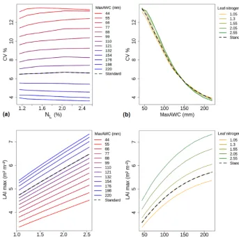
Figure 3 presents the impact of ISBA parameters on the sim-ulated annual maximum LAI and on its interannual variabil-ity. Two key parameters are considered: MaxAWC andNL. The same parameter values are applied to all 45 départe-ments, and mean modelled LAImaxare used to calculate CV values (Eq. 10). The CV values are shown in Fig. 3 as a func-tion of these parameters, together with LAImax.

It appears that the interannual variability of the modelled LAImaxis governed by MaxAWC. The CV values of more than 12 % are derived from the ISBA simulations at low val-ues of MaxAWC (e.g. 50 mm). On the other hand, high Max-AWC values (>200 mm) correspond to limited interannual variability of LAImax(CV<4 %), in relation to a lower sen-sitivity of plants to drought.

Figure 3.Impact of MaxAWC andNLparameters on the annual maximum LAI simulated by ISBA and on its interannual variability. The interannual variability is quantified using the coefficient of variation (CV, in %). Mean CV values (across all 45 départements) are plotted as a function of(a)NLand(b)MaxAWC, for various values of MaxAWC andNL, respectively. Mean LAImaxvalues (across all 45 départements) are plotted as a function of(c)NLand(d)MaxAWC, for various values of MaxAWC andNL, respectively. The dashed lines are obtained using standard average ISBA parameter values (MaxAWC=132 mm andNL=1.3 %).

at highNLvalues. SwitchingNLfrom low to high values at a given MaxAWC level also raises LAImax, but not more than 2 m2m−2.

This result confirms that MaxAWC is the key parameter to be retrieved in order to improve the representation of straw cereal biomass, for both inverse modelling and LDAS tuning experiments. The impact of MaxAWC on the cost functions (LAI RMSE and median LAI analysis increments, Eqs. 11 and 2, respectively) may depend on the LAI observation pe-riod. We tested the two retrieval methods for three different optimisation periods: start of growing period, peak LAI and senescence (see Sect. 2.7).

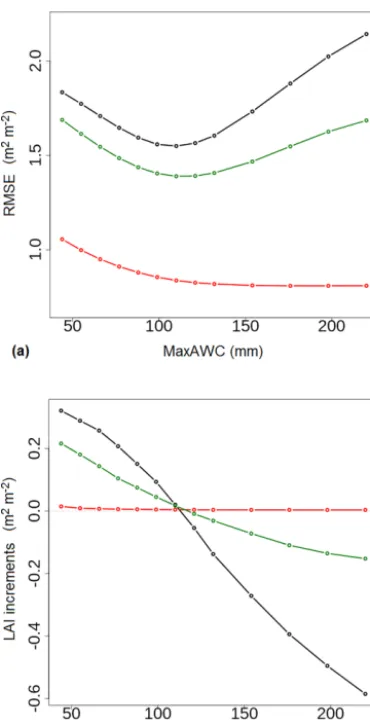
This is illustrated in Fig. 4, which shows the average cost function across all 45 départements. In both experiments, MaxAWC has little impact on the cost function during the start of the growing season. The most pronounced response of both LAI RMSE and analysis increments is observed dur-ing the senescence. For this period of the growdur-ing cycle, both cost functions present a minimum value at MaxAWC

=110 mm. Also, the largest RMSE and increment values are observed during senescence, indicating that the processes at stake during this period are more difficult to simulate. For straw cereals, senescence is related to soil moisture stress (Cabelguenne and Debaeke, 1998) and during this period the value of MaxAWC has a marked impact on the representation of the effect of drought by the model. The peak LAI period is less favourable to the integration of LAI observations into the model, with a reduced accuracy on the retrieved MaxAWC. 3.3 Outcomes of the optimisation

Figure 4. Mean cost function values vs. MaxAWC across all 45 départements of(a)inverse modelling and(b)LDAS tuning experi-ments for three different optimisation periods: (red) start of growing period (from 1 March to LAImaxdate); (green) peak LAI (dates for which LAI>0.5 LAImax); (black) senescence (from LAImaxdate to 31 July). Inverse modelling is based on the minimisation of LAI RMSE (Eq. 11). LDAS tuning is based on the minimisation of the median LAI analysis increment (Eq. 2).

The RMSE values are systematically reduced by the in-verse modelling experiment. For all 45 départements, the me-dian value of the LAI RMSE drops from 1.6 to 1.2 m2m−2. While LAI RMSE exceeds 1.5 m2m−2for 29 départements before the optimisation, this RMSE value is exceeded for only three départements after the optimisation. It must be noted that this is a much better result than the RMSE ob-tained in Fig. 4 (1.6 m2m−2)for the cost function including all 45 départements, with a MaxAWC value of 110 mm. This shows the impact of the spatial variability of MaxAWC.

For LDAS tuning, most of the median daily increment val-ues are sharply reduced: while 17 valval-ues are larger (smaller) than 0.2 (−0.2) m2m−2before the optimisation, all the val-ues range from −0.1 to 0.1 m2m−2 after the optimisation.

Figure 5. Cost function values during the senescence period af-ter vs. before LAI observation integration for all 45 départements: (a)LAI RMSE (Eq. 11) for inverse modelling and(b)LAI analysis increments (Eq. 2) for LDAS tuning. Identity lines are in blue.

The spatial median value of the LDAS LAI increments varies from−0.03 m2m−2for original LDAS to−0.01 m2m−2for LDAS tuning, for all 45 départements. Table 1 summarises results showing the impact of the optimisation on indicators such as the number of départements presenting a significant correlation ofBagXwith GY and the median value of the cost

functions. Table 2 also gives median and standard deviation values of the retrieved MaxAWC and of the retrievedNLin the case of inverse modelling, together with modelledBagX

and LAImax values. The results are given for the départe-ments presenting a significant correlation ofBagXwith GY

and for all 45 départements. An extended version of Table 1 (Table S3 in the Supplement) also gives results for undis-aggregated LAI and for 15 validated départements for both inverse modelling and LDAS tuning.

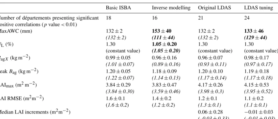
Table 1. Impact of the optimisation (either inverse modelling or LDAS tuning) on parameter values (spatial median values±standard deviation) of the ISBA model (MaxAWC andNL), on the median value ofBagXand LAImax, on peak simulatedBagand on the models scores during the senescence period with respect to the disaggregated LAI observations. The results are given for the validated départements, i.e. those presenting a significant correlation (pvalue<0.01) ofBagXwith Agreste straw cereal grain yield observations. Results for all 45

départements are given in brackets and in italics. Parameter values resulting from the optimisation are in bold. Because simulated LAImax andBagXvary from one year to another, spatial median values are based on median temporal values across the considered 15-year period.

Basic ISBA Inverse modelling Original LDAS LDAS tuning

Number of départements presenting significant positive correlations (pvalue<0.01)

18 16 21 24

MaxAWC (mm) 132±2 (132±2)

153±40 (111±44)

132±2 (132±2)

133±46 (129±44)

NL(%) 1.30

(constant value)

1.05±0.20 (1.05±0.20)

1.30

(constant value)

1.30

(constant value)

BagX(kg m−2) 0.99±0.05

(1.01±0.07)

0.96±0.16 (0.89±0.16)

0.96±0.07 (0.93±0.11)

0.98±0.17 (0.97±0.17) PeakBag(kg m−2) 1.20±0.05

(1.22±0.07)

1.18±0.09 (1.14±0.13)

1.20±0.10 (1.17±0.14)

1.19±0.18 (1.17±0.18) LAImax(m2m−2) 3.84±0.29

(3.84±0.30)

3.83±0.47 (3.59±0.46)

4.17±0.26 (3.98±0.3)

4.15±0.53 (3.95±0.52) LAI RMSE (m2m−2) 1.6±0.1

(1.6±0.2)

1.4±0.2 (1.2±0.2)

1.2±0.1 (1.3±0.1)

1.1±0.2 (1.1±0.1) Median LAI increments (m2m−2) 0.06±0.28

(–0.03±0.33)

−0.01±0.03 (–0.01±0.03)

Table 2.Impact ofNLon MaxAWC retrieval using a single-parameter inverse modelling technique. The retrieved median MaxAWC and LAI RMSE are given for all 45 départements together with their standard deviation.

NL(%) 1.05 1.30 1.55 2.05 2.55

Number of départements presenting significant positive correlations (pvalue<0.01)

16 13 12 6 3

MaxAWC (mm) 110±44 110±44 99±43 99±41 88±40 LAI RMSE (m2m−2) 1.2±0.2 1.2±0.2 1.3±0.2 1.4±0.2 1.5±0.2

133±46 mm for significant départements) is close to the standard value used in ISBA (132±2 mm) but the standard deviation is much larger. This shows that LDAS tuning is able to generate spatial variability in MaxAWC values.

A similar degree of variability is obtained by inverse mod-elling, but the retrieved MaxAWC presents much lower val-ues for all 45 départements: 111±44 mm. On the other hand, a much larger value of 153±40 mm is found for the 16 validated départements. The retrieved NL (1.05±0.20) is smaller than the default value of 1.30 %. The role of NLin the optimisation is discussed in Sect. 4.1.

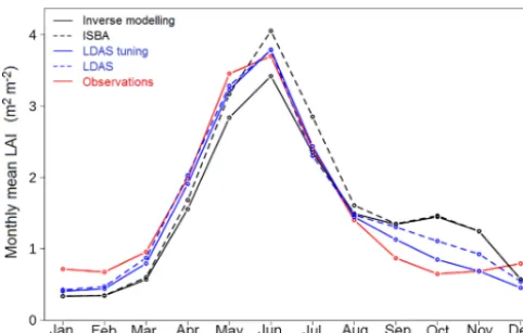
Figure 6 shows the impact of optimising MaxAWC on the mean annual LAI cycle, with respect to the observed annual LAI cycle over the 45 départements. Inverse modelling tends to produce a smaller LAImaxmedian value (3.59 m2m−2for all 45 départements) than basic ISBA simulations or LDAS simulations (3.84 and 3.98 m2m−2, respectively). Inverse modelling tends to reduce simulated LAI in May and June,

while the LDAS simulations (either original LDAS or LDAS tuning) are much closer to the observations.

The two optimisation methods succeed in reducing the LAI RMSE of the basic ISBA simulations (1.6 m2m−2 for all 45 départements). With optimised MaxAWC, the tuned LDAS annual mean LAI cycle is closer to the observations than LAI resulting from inverse modelling, with LAI RMSE equal to 1.1 m2m−2for LDAS tuning, as against 1.2 m2m−2 for inverse modelling.

3.4 Validation

Agricultural GY statistics (Sect. 2.3) are used for validation. The optimisation is considered as successful in départements where the correlation between yearly time series ofBagXand

Figure 6.Mean LAI annual cycle of straw cereals over France (45 départements) during the 1999–2013 period: satellite-derived obser-vations (red line); basic ISBA simulation (dark dashed line); origi-nal LDAS simulation (blue dashed line); inverse modelling simula-tion (solid dark line); LDAS tuning simulasimula-tion (solid blue line).

24 départements. With only 16 validated départements, in-verse modelling is not able to outperform the original LDAS simulations.

Time series of mean scaled anomalies of BagX and GY

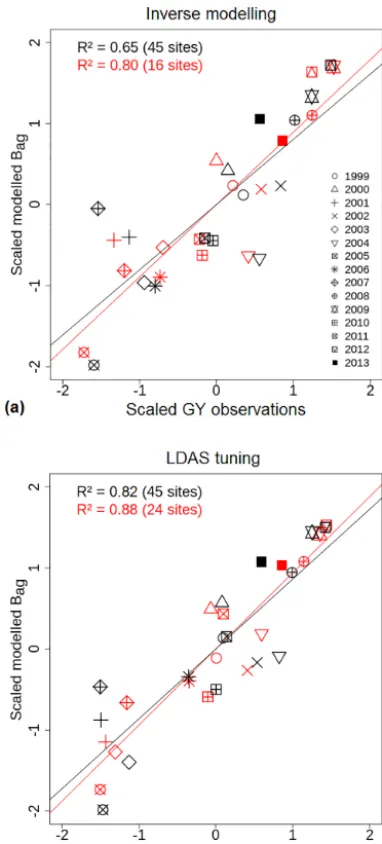
are shown in Fig. 7 for all 45 départements before and af-ter inverse modelling or LDAS tuning. The marked nega-tive anomalies (<−1) in 2001, 2003 and 2011 are repre-sented well after LDAS tuning. On the other hand, the impact of sunlight deficit and low temperatures during the grow-ing period of 2001 cannot be represented well after inverse modelling. The marked negative GY anomaly observed in 2007 is not very well represented by the model. Moreover, Fig. 7 shows that parameter tuning does not significantly im-proveR2values. Basic ISBA and original LDAS simulations presentR2values of 0.65 and 0.80, as against 0.65 and 0.82 after inverse modelling and LDAS tuning, respectively.

Figure 8 further shows that the interannual variability of BagXis markedly better represented using LDAS tuning. The

scaled modelledBagXand the scaled GY observations

aver-aged over 45 départements present aR2value of 0.82, against 0.65 for inverse modelling. Considering only the success-fully validated départements, more similarR2values are ob-served: 0.88 and 0.80, respectively. Figure 9 presents the spa-tial correlation between the scaled BagX and the scaled GY

observations averaged over the 15-year period considered in this study. Considering the 45 départements,R2=0.61 for LDAS tuning and R2=0.58 for inverse modelling. Again, LDAS tuning supersedes inverse modelling, including when the comparison is limited to successfully validated départe-ments, withR2values of 0.74 and 0.63, respectively.

It must be noted that all the correlations presented in Figs. 8 and 9 are significant, with allp values smaller than 0.001.

In addition to GY data, we made an attempt to use the satellite-derived GLEAM evapotranspiration product

(Mi-Figure 7.Scaled GY observation anomalies (AsGY)and scaled

sim-ulatedBagXanomalies (AsBagX)after LAI observation integration

for all 45 départements:(a)inverse modelling and(b)LDAS tuning. Red lines are for observations, dark lines are for simulations, dark dashed line is for the original un-tuned simulations. The fraction of explained variance byAsBagX isR2=0.65 for inverse modelling,

and 0.82 for LDAS tuning.

ralles et al., 2011) but very poor correlations were obtained for most départements (the medianR2 value was less than 0.06). On the other hand, good correlations were found for photosynthesis using the GPP FLUXNET-MTE product de-scribed in Jung et al. (2009). With respect to basic ISBA sim-ulations, GPP RMSE was nearly systematically improved by the original LDAS simulations, and LDAS tuning drastically reduced the largest RMSE values, observed in southwestern France (see Figs. S2 and S3 in the Supplement).

3.5 Impact of the optimisation technique on MaxAWC estimates

Figure 8.Temporal correlation betweenAsBagX andAsGY for (red

symbols) départements presenting significant positive correlations (p value<0.01) between simulated BagX and GY and (red and

black symbols) all 45 départements, and for(a)inverse modelling and(b)LDAS tuning.

The similarity in MaxAWC estimates and the contrasting simulated LAI values are illustrated in Fig. 10. Analysed LAI from LDAS tuning is closer to the LAI observations than the simulated LAI resulting from inverse modelling. The Max-AWC estimates are slightly smaller for inverse modelling and correlate very well with the MaxAWC estimates from LDAS tuning (R2=0.81). The latter result is also valid when all 45 départements are considered, withR2=0.72.

Figure 9.As in Fig. 8, except for spatial correlation.

4 Discussion

4.1 What is the added value of the LDAS?

Figure 10.Inverse modelling vs. LDAS tuning:(a)mean LAI an-nual cycle for 15 validated départements with both methods from satellite-derived observations (red line), inverse modelling (dark line) and LDAS tuning (blue line);(b)MaxAWC comparison for (+) all 45 départements (R2=0.72) and for (red circles) the 15 common départements (R2=0.81).

LDAS to use the observations to drive the model trajectory: the sequential assimilation of LAI is able to constrain the simulated LAI values.

It can be shown that the impact of tuningNLin the inverse modelling method can be significant. Table 2 presents Max-AWC and LAI RMSE values obtained from inverse mod-elling when only one parameter, MaxAWC, is optimised. Re-sults are shown for five values of NL ranging from 1.05 to 2.55 %. The number of validated départements drops when NL increases, from 16 at NL=1.05 % to only 3 at NL= 2.55 %. At the same time, the MaxAWC estimates tend to present smaller values, down to 88±40 mm atNL=2.55 %. This result can be explained by the fact that larger values of either MaxAWC orNLtend to increase LAImax(Fig. 3).

Improving the simulation of vegetation variables has a positive impact on the quality of simulated hydrological vari-ables such as evapotranspiration and soil moisture (Szczypta et al., 2012). Therefore, the larger MaxAWC values ob-tained from LDAS tuning (129±44 mm) are likely to be more realistic than those obtained from inverse modelling (111±44 mm).

4.2 Are MaxAWC estimates and simulated peakBag

realistic?

Independent MaxAWC estimates confirm that the Max-AWC values obtained from LDAS tuning (129±44 mm) are more realistic than those obtained from inverse modelling (111±44 mm). On the other hand, the two techniques give similar medianBagXvalues (Table 1).

In order to verify the MaxAWC values derived from LAI observations, we extracted MaxAWC values from a map pro-duced by l’Institut National de la Recherche Agronomique (INRA) at a spatial resolution of 1 km×1 km. This map was established using pedotransfer functions based on soil phys-ical properties information such as soil texture, soil depth, bulk density and organic matter (Al Majou et al., 2008). A given local MaxAWC value corresponds to a soil ty-pological unit (STU). The 1 km×1 km soil mapping units may contain several STUs and the STU fraction is known. We computed weighted-average MaxAWC values for every 35×35 km grid cell. The resulting INRA MaxAWC values of the 45 départements present a median value of 151 mm and a standard deviation of 54 mm.

The median peakBag values are about 1.2 kg m−2 in all simulations. This is consistent with total maximum above-ground biomass values for cereals, which range between 1.1 and 1.7 kg m−2(e.g. Loubet et al., 2011). BecauseBagX

cor-responds to the meanBagabove 90 % of the peakBagvalue (Sect. 2.7), medianBagX values are smaller than peakBag and do not exceed 1 kg m−2(Table 1).

4.3 Are LAI satellite data suitable for the optimisation of MaxAWC?

Our results show that using disaggregated LAI observations is key.

The optimisation methods used in this study are based on disaggregated LAI satellite data and the quality of the results depends on the reliability of the observation data set. The MaxAWC parameter is a crucial parameter for the senescence period, between LAImaxand harvesting (Fig. 4). Because LAImax is related to a large extent to MaxAWC (Fig. 3d), an underestimation of observed maximum LAI val-ues would force the retrieval method to underestimate Max-AWC.

Figure 11.Comparison of mean annual LAImaxof the raw GEOV1 product and of the disaggregated GEOV1 product.

LAI increases the observed value of maximum LAI by up to 40 % with respect to raw LAI. The mean difference is 0.43 m2m−2. This mitigates a marked underestimation of the MaxAWC estimates. As shown in Table S3, the MaxAWC values obtained from LDAS tuning (110±38 mm) and from inverse modelling (83±30 mm) are much lower (15 to 25 %) than those retrieved using disaggregated LAI observations. Moreover, the number of validated départements using GY observations presenting significant positive correlation is re-duced: only 10 and 18 for inverse modelling and LDAS tun-ing, as against 16 and 24 with disaggregated LAI, respec-tively. Also, peak Bag values (for all 45 départements) are smaller: 1.01 and 1.08 kg m−2, against 1.14 and 1.17 kg m−2 with disaggregated LAI, respectively.

4.4 Can model simulations predict the relative gain or loss of agricultural production during extreme years?

The continuous constraint on the model applied by the LDAS on simulated vegetation variables allows the indirect repre-sentation of adverse effects. This is illustrated in Fig. 7: the negative anomaly of 2007 is much better represented by the LDAS than by simple ISBA simulations.

The observed disaggregated LAI and GY in Fig. 2 show that 2004, 2008, 2009 and 2012 were favourable years for straw cereal production, while 2001, 2003, 2007 and 2011 were unfavourable years. Unfavourable conditions for straw cereal production were caused by droughts, by excess of wa-ter, or by a deficit in solar radiation. For example, the 2000– 2001 winter was characterised by extensive floods and by a deficit of solar irradiance until the end of the spring. These climate events markedly affected plant growth especially in

Figure 12.Use of median observed annual maximum of LAI to retrieve MaxAWC for all 45 départements:(a) linear regression relationship between maximum LAI and the LDAS tuning Max-AWC estimates;(b)MaxAWC estimates derived from the statisti-cal model using maximum LAI observations as a predictor vs. the LDAS tuning MaxAWC estimates.

4.5 Can observed LAI characteristics be used to estimate MaxAWC?

We show that satellite-derived LAI observations have poten-tial to map MaxAWC very simply.

We investigated the use of a simple statistical analysis of the disaggregated LAI observations to estimate MaxAWC. Figure 3 shows that there is a marked relationship between MaxAWC and the simulated LAImaxand LAI CV. To what extent are these relationships observable?

In order to answer this question, we used the LDAS tun-ing MaxAWC estimates as a reference data set. We compared the observed median annual maximum LAI and LAI CV with MaxAWC. No significant correlation could be shown for LAI CV, withR2smaller than 0.2. On the other hand, a very good correlation (R2=0.70 for all 45 départements) was found for median annual maximum LAI (Fig. 12). Using this sim-ple linear regression model, MaxAWC can be estimated with a RMSE of 28.7 mm. A very similar result is obtained con-sidering only the 24 validated départements for LDAS tun-ing. The modelled MaxAWC values are given in Table S2 (see Supplement).

5 Conclusions

Satellite data are used to optimise a key parameter of the ISBA land surface model for straw cereals in France: the maximum available soil water content, MaxAWC. Two op-timisation methods are used. Inverse modelling consists in minimising the LAI RMSE and LDAS tuning consists in minimising LAI analyses increments. The added value of the optimisation is evaluated using simulated above-ground biomass, through its correlation with in situ grain yield ob-servations.

It is found that disaggregated LAI observations during the senescence are more informative than raw LAI observations and than LAI observations during the growing phase. The best results are obtained using LDAS tuning: the simulated above-ground biomass correlates better with grain yield ob-servations, and the retrieved MaxAWC values are more real-istic. It is shown that LDAS simulations can predict the rel-ative gain or loss of agricultural production during extreme years, much better than model simulations even after param-eter optimisation.

Finally, it is shown that median annual maximum dis-aggregated LAI observations correlate with MaxAWC esti-mates over France. This simple metric derived from LAI ob-servations could be used to map MaxAWC. More research is needed to investigate to what extent this conclusion holds for other regions of the world and other vegetation types.

Appendix A: Nomenclature List of symbols

As,BagX Scaled anomaly ofBagXof a given year (–)

As,GY Scaled anomaly of GY of a given year (zscore) (–) AWC Simulated available soil water content (kg m−2)

Bag Simulated living above-ground biomass (kg of dry matter m−2)

BagX Maximum of simulated living above-ground biomass (kg of dry matter m−2)

CV Coefficient of variation (%)

Dmax Maximum leaf-to-air saturation deficit (kg kg−1)

Fs Soil moisture stress function

gm Mesophyll conductance in well-watered conditions (mm s−1) GY Annual grain yields of crops (kg m−2)

LAI Leaf area index (m2m−2)

LDAS Land data assimilation system

LSM Land surface model

MaxAWC Maximum available soil water content (mm or kg m−2) NIT Photosynthesis-driven plant growth version of ISBA-A-gs NL Leaf nitrogen concentration (% of leaf dry mass)

SLA Specific leaf area (m2kg−1)

WUE Leaf-level water use efficiency (ratio of net assimilation of CO2to leaf transpiration)

Zr Depth of the root zone layer (m)

Greek symbols

ρ Water density (kg m−3)

θ Volumetric soil water content (m3m−3₎

The Supplement related to this article is available online at https://doi.org/10.5194/hess-21-4861-2017-supplement.

Competing interests. The authors declare that they have no conflict of interest.

Acknowledgements. The work of Hélène Dewaele was supported by CNES and by Météo-France. The work of Simon Munier was supported by European Union Seventh Framework Programme (FP7/2007–2013) under grant agreement no. 603608, “Global Earth Observation for integrated water resource assessment” (eartH2Observe). The work of Nabil Laanaia was supported by the Belgian MASC BELSPO project under contract no. BR/121/A2/MASC. The authors would like to thank the Coper-nicus Global Land service for providing the satellite-derived LAI products.

Edited by: Hannah Cloke

Reviewed by: two anonymous referees

References

Agreste: Annual statistical surveys over France, available at: http:// agreste.agriculture.gouv.fr/ (last access: September 2017), 2015. Agreste Bilans: Agreste, Publications, Chiffres et Données No. 11, Bilan conjoncturel de l’année agricole 2001, 16 pp., available at: www.agreste.agriculture.gouv.fr/IMG/pdf/BILAN2001NOTE. pdf (last access: February 2017), 2001.

Agreste Bilans: Agreste, Publications, Chiffres et Données Agricul-ture, Bilan conjoncturel Novembre 2003, 2 pp., available at: http: //agreste.agriculture.gouv.fr/IMG/pdf/conjenc10311.pdf (last ac-cess: February 2017), 2003.

Agreste Bilans: Agreste, Publications, Chiffres et Données No. 10–11, Bilan conjoncturel 2007, 40 pp., available at: www. agreste.agriculture.gouv.fr/IMG/pdf/bilan2007note.pdf (last ac-cess: February 2017), 2007.

Agreste Bilans: Agreste, Publications, Chiffres et Données Agricul-ture No. 7, Bilan conjoncAgricul-turel 2011, 45 pp., available at: www. agreste.agriculture.gouv.fr/IMG/pdf_bilan2011note.pdf (last ac-cess: February 2017), 2011.

Albergel, C., Calvet, J.-C., Mahfouf, J.-F., Rüdiger, C., Barbu, A. L., Lafont, S., Roujean, J.-L., Walker, J. P., Crapeau, M., and Wigneron, J.-P.: Monitoring of water and carbon fluxes us-ing a land data assimilation system: a case study for south-western France, Hydrol. Earth Syst. Sci., 14, 1109–1124, https://doi.org/10.5194/hess-14-1109-2010, 2010.

Al Majou, H., Bruand, A., Duval, O., Le Bas, C., and Vauer, A.: Prediction of soil water retention properties after stratification by combining texture, bulk density and the type of horizon, Soil Use Manage., 24, 383–391, https://doi.org/10.1111/j.1475-2743.2008.00180.x, 2008.

Barbu, A. L., Calvet, J.-C., Mahfouf, J.-F., Albergel, C., and Lafont, S.: Assimilation of Soil Wetness Index and Leaf Area Index into the ISBA-A-gs land surface model: grassland case study,

Bio-geosciences, 8, 1971–1986, https://doi.org/10.5194/bg-8-1971-2011, 2011.

Barbu, A. L., Calvet, J.-C., Mahfouf, J.-F., and Lafont, S.: Integrat-ing ASCAT surface soil moisture and GEOV1 leaf area index into the SURFEX modelling platform: a land data assimilation application over France, Hydrol. Earth Syst. Sci., 18, 173–192, https://doi.org/10.5194/hess-18-173-2014, 2014.

Baret, F., Weiss, M., Lacaze, R., Camacho, F., Makhmara, H., Pa-cholczyk, P., and Smets, B.: GEOV1: LAI and FAPAR essen-tial climate variables and FCOVER global time series capitaliz-ing over existcapitaliz-ing products, Part 1: Principles of development and production, Remote Sens. Environ., 137, 299–309, 2013. Bastos, A., Gouveia, C. M., Trigo, R. M., and Running, S. W.:

Analysing the spatio-temporal impacts of the 2003 and 2010 extreme heatwaves on plant productivity in Europe, Biogeo-sciences, 11, 3421–3435, https://doi.org/10.5194/bg-11-3421-2014, 2014.

Becker-Reshef, I., Vermote, E., Lindeman, M., and Justice, C.: A generalized regression-based model for forecasting winter wheat yields in Kansas and Ukraine using MODIS data, Remote Sens. Environ., 114, 1312–1323, 2010.

Cabelguenne, M. and Debaeke, P.: Experimental determination and modelling of the soil water extraction capacities of crops of maize, sunflower, soya bean, sorghum and wheat, Plant Soil, 202, 175–192, https://doi.org/10.1023/A:1004376728978, 1998. Calvet, J.-C.: Investigating soil and atmospheric plant water stress

using physiological and micrometeorological data, Agr. Forest Meteorol., 103, 229–247, 2000.

Calvet, J.-C. and Soussana, J.-F.: Modelling CO2-enrichment ef-fects using an interactive vegetation SVAT scheme, Agr. Forest Meteorol., 108, 129–152, 2001.

Calvet, J.-C., Noilhan, J., Roujean, J., Bessemoulin, P., Ca-belguenne, M., Olioso, A., and Wigneron, J.: An interactive veg-etation SVAT model tested against data from six contrasting sites, Agr. Forest Meteorol., 92, 73–95, 1998.

Calvet, J.-C., Gibelin, A.-L., Roujean, J.-L., Martin, E., Le Moigne, P., Douville, H., and Noilhan, J.: Past and future scenarios of the effect of carbon dioxide on plant growth and transpi-ration for three vegetation types of southwestern France, At-mos. Chem. Phys., 8, 397–406, https://doi.org/10.5194/acp-8-397-2008, 2008.

Calvet, J.-C., Lafont, S., Cloppet, E., Souverain, F., Badeau, V., and Le Bas, C.: Use of agricultural statistics to verify the interannual variability in land surface models: a case study over France with ISBA-A-gs, Geosci. Model Dev., 5, 37-54, https://doi.org/10.5194/gmd-5-37-2012, 2012.

Canal, N., Calvet, J.-C., Decharme, B., Carrer, D., Lafont, S., and Pigeon, G.: Evaluation of root water uptake in the ISBA-A-gs land surface model using agricultural yield statis-tics over France, Hydrol. Earth Syst. Sci., 18, 4979–4999, https://doi.org/10.5194/hess-18-4979-2014, 2014.

Capa-Morocho, M., Rodriguez-Fonseca, B., and Ruiz-Ramoz, M.: Crop yields as a bioclimatic index of El Nino impact in Europe: Crop forecast implications, Agr. Forest Meteorol., 198–199, 42– 52, https://doi.org/10.1016/j.agrformet.2014.07.012, 2014. Carrer, D., Roujean, J.-L., Lafont, S., Calvet, J.-C., Boone,

im-pact on carbon fluxes, J. Geophys. Res.-Biogeo., 118, 1–16, https://doi.org/10.1002/jgrg.20070, 2013.

Carrer, D., Meurey, C., Ceamanos, X., Roujean, L., Calvet, J.-C., and Liu, S.: Dynamic mapping of snow-free vegetation and bare soil albedos at global 1 km scale from 10-year analysis of MODIS satellite products, Remote Sens. Environ., 140, 420– 432, https://doi.org/10.1016/j.rse.2013.08.041, 2014.

Copernicus: LAI GEOV1, available at: http://land.copernicus.eu/ global/ (last access: September 2017), 2015.

Crow, W. T., Kumar, S. V., and Bolten, J. D.: On the utility of land surface models for agricultural drought monitoring, Hydrol. Earth Syst. Sci., 16, 3451–3460, https://doi.org/10.5194/hess-16-3451-2012, 2012.

Dee, D. P., Uppala, S. M., Simmons, A. J., Berrisford, P., Poli, P., Kobayashi, S., Andrae, U., Balmaseda, M. A., Balsamo, G., Bauer, P., Bechtold, P., Beljaars, A. C. M., van de Berg, L., Bid-lot, J., Bormann, N., Delsol, C., Dragani, R., Fuentes, M., Geer, A. J., Haimberger, L., Healy, S. B., Hersbach, H., Hólm, E. V., Isaksen, L., Kallberg, P., Köhler, M., Matricardi, M., McNally, A. P., Monge-Sanz, B. M., Morcrette, J. J., Park, B. K., Peubey, C., de Rosnay, P., Tavolato, C., Thépaut, J.-N., and Vitart, F.: The ERA-Interim reanalysis: configuration and performance of the data assimilation system, Q. J. Roy. Meteor. Soc., 137, 553–597, https://doi.org/10.1002/qj.828, 2011.

Eitzinger, J., Trnka, M., Hösch, J., Žalud, Z., and Dubrovský, M.: Comparison of CERES, WOFOST and SWAP models in simulating soil water content during growing season un-der different soil conditions, Ecol. Model., 171, 223–246, https://doi.org/10.1016/j.ecolmodel.2003.08.012, 2004. Faroux, S., Kaptué Tchuenté, A. T., Roujean, J.-L., Masson, V.,

Martin, E., and Le Moigne, P.: ECOCLIMAP-II/Europe: a twofold database of ecosystems and surface parameters at 1 km resolution based on satellite information for use in land surface, meteorological and climate models, Geosci. Model Dev., 6, 563– 582, https://doi.org/10.5194/gmd-6-563-2013, 2013.

Ferrant, S., Gascoin, S., Veloso, A., Salmon-Monviola, J., Claverie, M., Rivalland, V., Dedieu, G., Demarez, V., Ceschia, E., Probst, J.-L., Durand, P., and Bustillo, V.: Agro-hydrology and multi-temporal high-resolution remote sensing: toward an explicit spa-tial processes calibration, Hydrol. Earth Syst. Sci., 18, 5219– 5237, https://doi.org/10.5194/hess-18-5219-2014, 2014. Folberth, C., Skalsky, R., Moltchanova, E., Balkovic, J., Azevedo,

L. B., Obersteiner, M., and van der Velde, M.: Uncer-tainty in soil data can outweigh climate impact signals in global crop yield simulations, Nat. Commun., 7, 11872, https://doi.org/10.1038/ncomms11872, 2016.

Ford, T. W., Harris, E., and Quiring, S. M.: Estimating root zone soil moisture using near-surface observations from SMOS, Hy-drol. Earth Syst. Sci., 18, 139–154, https://doi.org/10.5194/hess-18-139-2014, 2014.

Ghilain, N., Arboleda, A., Sepulcre-Cantò, G., Batelaan, O., Ardö, J., and Gellens-Meulenberghs, F.: Improving evapotranspiration in a land surface model using biophysical variables derived from MSG/SEVIRI satellite, Hydrol. Earth Syst. Sci., 16, 2567–2583, https://doi.org/10.5194/hess-16-2567-2012, 2012.

Gibelin, A.-L., Calvet, J.-C., Roujean, J.-L., Jarlan, L., and Los, S. O.: Ability of the land surface model ISBA-A-gs to simulate leaf area index at the global scale:

Compari-son with satellites products, J. Geophys. Res., 111, D18102, https://doi.org/10.1029/2005JD006691, 2006.

Ichii, K., Wang, W., Hashimoto, H., Yang, F., Votava, P., Michaelis., A. R., and Nemani, R. R.: Refinement of rooting depths us-ing satellite based evapotranspiration seasonality for ecosystem modelling in California, Agr. Forest Meteorol., 149, 1907–1918, 2009.

Jung, M., Reichstein, M., and Bondeau, A.: Towards global empirical upscaling of FLUXNET eddy covariance obser-vations: validation of a model tree ensemble approach using a biosphere model, Biogeosciences, 6, 2001–2013, https://doi.org/10.5194/bg-6-2001-2009, 2009.

Kowalik, W., Dabrowska-Zielinska, K., Meroni, M., Raczka, U. T., and de Wit A.: Yield estimation using SPOT-VEGETATION products: A case study of wheat in Euro-pean countries, Int. J. Appl. Earth Obs. Geoinf., 32, 228–239, https://doi.org/10.1016/j.jag.2014.03.011, 2014.

Krinner, G., Viovy, N., de Noblet-Ducoudré, N., Ogée, J., Polcher, J., Friedlingstein, P., Ciais, P., Sitch, S., and Prentice, I. C.: A dynamic global vegetation model for studies of the cou-pled atmosphere-biosphere system, Global Biogeochem. Cy., 19, GB1015, https://doi.org/10.1029/2003GB002199, 2005. Li, S., Wheeler, T., Challinor, A., Lin, E., Ju, H., and

Xu, Y.: The observed relationship between wheat and cli-mate in China, Agr. Forest Meteorol., 150, 1412–1419, https://doi.org/10.1016/j.agrformet.2010.07.003, 2010.

Loubet, B., Laville, P. Lehuger, S., Larmanou, E., Fléchard C., Mascher N., Genermont S., Roche R., Ferrara, R. M., Stella, P., Personne, E., Durand B., Decuq C., Flura, D., Mas-son, S., Fanucci, O., Rampon, J.-N., Siemens, J., Kindler, R., Gabrielle B., Schrumpf, M., and Cellier P.: Carbon, ni-trogen and Greenhouse gases budgets over a four years crop rotation in northern France, Plant Soil, 343, 109–137, https://doi.org/10.1007/s11104-011-0751-9, 2011.

Masson, V., Le Moigne, P., Martin, E., Faroux, S., Alias, A., Alkama, R., Belamari, S., Barbu, A., Boone, A., Bouyssel, F., Brousseau, P., Brun, E., Calvet, J.-C., Carrer, D., Decharme, B., Delire, C., Donier, S., Essaouini, K., Gibelin, A.-L., Giordani, H., Habets, F., Jidane, M., Kerdraon, G., Kourzeneva, E., Lafaysse, M., Lafont, S., Lebeaupin Brossier, C., Lemonsu, A., Mahfouf, J.-F., Marguinaud, P., Mokhtari, M., Morin, S., Pigeon, G., Sal-gado, R., Seity, Y., Taillefer, F., Tanguy, G., Tulet, P., Vincendon, B., Vionnet, V., and Voldoire, A.: The SURFEXv7.2 land and ocean surface platform for coupled or offline simulation of earth surface variables and fluxes, Geosci. Model Dev., 6, 929–960, https://doi.org/10.5194/gmd-6-929-2013, 2013.

Miralles, D. G., Holmes, T. R. H., De Jeu, R. A. M., Gash, J. H., Meesters, A. G. C. A., and Dolman, A. J.: Global land-surface evaporation estimated from satellite-based observations, Hydrol. Earth Syst. Sci., 15, 453–469, https://doi.org/10.5194/hess-15-453-2011, 2011.

Munier, S., Carrer, D., Planque, C., Camacho, F., Albergel, C., and Calvet, J.-C.: Satellite Leaf Area Index: global scale analysis of the tendencies per vegetation type over the last 17 years, Remote Sens. Environ., submitted, 2017.

2012, available at: http://webarchive.iiasa.ac.at/Research/LUC/ External-World-soil-database/HWSD_Documentation.pdf (last access: December 2014), 2012.

Olesen, J. E., Trnka, M., Kersebaum, K. C., Skjelvag, A. O., Seguin, B., Peltonen-Sainio, P., Rossi, F., Kozyra, J., and Mi-cale, F.: Impacts and adaptation of European crop production systems to climate change, Euro. J. Agronomy., 34, 96–112, https://doi.org/10.1016/j.eja.2010.11.003, 2011.

Piedallu, C., Gégout, J.-C., Bruand, A., and Seynave, I., Map-ping soil water holding capacity over large areas to predict po-tential production of forest stands, Geoderma, 160, 355–366, https://doi.org/10.1016/j.geoderma.2010.10.004, 2011.

Portoghese, I., Iacobellis, V., and Sivapalan, M.: Analysis of soil and vegetation patterns in semi-arid Mediterranean landscapes by way of a conceptual water balance model, Hydrol. Earth Syst. Sci., 12, 899–911, https://doi.org/10.5194/hess-12-899-2008, 2008.

Quiroga, S., Fernández-Haddad, Z., and Iglesias, A.: Crop yields response to water pressures in the Ebro basin in Spain: risk and water policy implications, Hydrol. Earth Syst. Sci., 15, 505–518, https://doi.org/10.5194/hess-15-505-2011, 2011.

Ritchie, J. T. and Otter, S.: Description and performance of CERES-wheat: A user-oriented wheat yield model, ARS wheat yield project, 38, 159–175, 1985.

Rüdiger, C., Albergel, C., Mahfouf, J.-F. , Calvet, J.-C., and Walker, J. P.: Evaluation of Jacobians for Leaf Area Index data assim-ilation with an extended Kalman filter, J. Geophys. Res., 115, D09111, https://doi.org/10.1029/2009JD012912, 2010. Soylu, M. E., Istanbulluoglu, E., Lenters, J. D., and Wang, T.:

Quan-tifying the impact of groundwater depth on evapotranspiration in a semi-arid grassland region, Hydrol. Earth Syst. Sci., 15, 787– 806, https://doi.org/10.5194/hess-15-787-2011, 2011.

Szczypta, C., Decharme, B., Carrer, D., Calvet, J.-C., Lafont, S., Somot, S., Faroux, S., and Martin, E.: Impact of precipitation and land biophysical variables on the simulated discharge of Eu-ropean and Mediterranean rivers, Hydrol. Earth Syst. Sci., 16, 3351–3370, https://doi.org/10.5194/hess-16-3351-2012, 2012.

Szczypta, C., Calvet, J.-C., Maignan, F., Dorigo, W., Baret, F., and Ciais, P.: Suitability of modelled and remotely sensed essential climate variables for monitoring Euro-Mediterranean droughts, Geosci. Model Dev., 7, 931–946, https://doi.org/10.5194/gmd-7-931-2014, 2014.

Tanaka, K., Takizawa, H., Kume, T., Xu, J., Tantasirin, C., and Suzuki, M.: Impact of rooting depth of soil hydraulic proper-ties on the transpiration peak of an evergreen forest in northern Thailand in the late dry season, J. Geophys. Res., 109, D23107, https://doi.org/10.1029/2004JD004865, 2004.

Van Dam, J. C., Huygen, J., Wesseling, J. G., Feddes, R. A., Kabat, P., Van Walsum, P. E. V., Groenendijk, P., and Van Diepen, C. A.: Theory of SWAP version 2.0. Simulation of water flow, solute transport and plant growth in the Soil–Water–Atmosphere–Plant environment, Report 71, Sub department of Water Resources, Wageningen University, Technical document, 45, 1997. Van Der Velde, M., Tubiello, N. F., Vrieling, A., and Bouraoui,

F.: Impacts of extreme weather on wheat and maize in France: evaluating regional crop simulations against observed data, Cli-matic Change, 113, 751–765, https://doi.org/10.1007/s10584-011-0368-2 2012.

Van Diepen, C. A., Wolf, J., Van Keulen, H., and Rappoldt, C.: WOFOST: a simulation model of crop production, Soil Use Man-age., 5, 16–24, 1989.

Wang, S., Fu, B. J., Gao, G. Y., Yao, X. L., and Zhou, J.: Soil mois-ture and evapotranspiration of different land cover types in the Loess Plateau, China, Hydrol. Earth Syst. Sci., 16, 2883–2892, https://doi.org/10.5194/hess-16-2883-2012, 2012.