https://doi.org/10.5194/hess-22-2759-2018 © Author(s) 2018. This work is distributed under the Creative Commons Attribution 4.0 License.
Effects of variability in probable maximum precipitation
patterns on flood losses
Andreas Paul Zischg1,2, Guido Felder1, Rolf Weingartner1, Niall Quinn3, Gemma Coxon2, Jeffrey Neal2, Jim Freer2, and Paul Bates2
1University of Bern, Institute of Geography, Oeschger Centre for Climate Change Research, Mobiliar Lab for Natural Risks,
Bern, 3012, Switzerland
2School of Geographical Sciences, University of Bristol, Bristol, BS8 1SS, UK 3Fathom Ltd., Bristol, BS1 6QF, UK
Correspondence:Andreas Paul Zischg ([email protected]) Received: 29 December 2017 – Discussion started: 31 January 2018 Revised: 19 April 2018 – Accepted: 24 April 2018 – Published: 8 May 2018
Abstract.The assessment of the impacts of extreme floods is important for dealing with residual risk, particularly for crit-ical infrastructure management and for insurance purposes. Thus, modelling of the probable maximum flood (PMF) from probable maximum precipitation (PMP) by coupling hydro-logical and hydraulic models has gained interest in recent years. Herein, we examine whether variability in precipita-tion patterns exceeds or is below selected uncertainty fac-tors in flood loss estimation and if the flood losses within a river basin are related to the probable maximum discharge at the basin outlet. We developed a model experiment with an ensemble of probable maximum precipitation scenarios created by Monte Carlo simulations. For each rainfall pat-tern, we computed the flood losses with a model chain and benchmarked the effects of variability in rainfall distribution with other model uncertainties. The results show that flood losses vary considerably within the river basin and depend on the timing and superimposition of the flood peaks from the basin’s sub-catchments. In addition to the flood hazard component, the other components of flood risk, exposure, and vulnerability contribute remarkably to the overall vari-ability. This leads to the conclusion that the estimation of the probable maximum expectable flood losses in a river basin should not be based exclusively on the PMF. Consequently, the basin-specific sensitivities to different precipitation pat-terns and the spatial organization of the settlements within the river basin need to be considered in the analyses of prob-able maximum flood losses.
1 Introduction
An important aspect in flood risk analysis is the modelling of worst-case floods and their impacts (Büchele et al., 2006). One main question herein is the search for the upper physi-cal limits of discharge in a river basin, i.e. the maximum out-flow from a catchment that is possible with the given catch-ment characteristics and the maximum rainfall in the cli-mate region (Felder and Weingartner, 2017). Here, the hydro-logical modelling undertaken to derive probable maximum flood (PMF) from probable maximum precipitation (PMP) is an important first step as a basis for inundation modelling (Felder et al., 2017). The PMP is defined as “the theoretical maximum precipitation for a given duration under modern meteorological conditions” (World Meteorological Organi-zation, 2009). Differently, the PMF is defined as “the theo-retical maximum flood that poses extremely serious threats to the flood control of a given project in a design water-shed” (World Meteorological Organization, 2009). The PMF is estimated on the basis of the PMP and is commonly used in practice for the planning of hydropower dams. However, there is still a controversial discussion on the underlying con-cept of PMP, particularly on the assumption that the upper tail of flood distributions is bounded (Micovic et al., 2015). Comprehensive summaries of this discussion are provided by Salas et al. (2015) and by Rouhani and Leconte (2016). Nev-ertheless, PMP/PMF estimation methods have been contin-uously developed and improved. Beauchamp et al. (2013), Lagos-Zuniga and Vargas (2014), and Felder and Weingart-ner (2016) discuss the role of the spatio-temporal distribu-tion of the PMP on the PMF, while Rousseau et al. (2014) and Stratz and Hossain (2014) discuss climate change and stationarity issues. Hence, Faulkner and Benn (2016), Mi-covic et al. (2015), Rouhani and Leconte (2016), and Salas et al. (2014) have proposed incorporating uncertainty bands into the PMP estimation.
Nevertheless, the detailed triggering mechanism and the temporal evolution of large flood events, specifically of worst-case scenarios, are not yet fully understood. An im-portant question concerns how the peak discharge and the volume of a flood depend on the intensity and track of the triggering precipitation events, i.e. the spatio-temporal pat-tern of precipitation (Adams et al., 2012; Bruni et al., 2015; Cristiano et al., 2017; Emmanuel et al., 2015, 2016; Ochoa-Rodriguez et al., 2015; Paschalis et al., 2014; Rafieeinasab et al., 2015; Zhang and Han, 2017). In addition to the storm track dynamics, the peak flow depends on the watershed characteristics (Singh, 1997). In mountainous catchments with high topographical complexity, the storm track and the precipitation pattern are influenced by the mountain ranges. Furthermore, the river network is influenced by geological and tectonic structures and is thus more complex in moun-tainous terrain than in low-lying areas. Thus, in upland areas high variability in the spatio-temporal pattern of a probable maximum precipitation event and the resulting river flows has to be assumed. The definition of the spatio-temporal characteristics of PMP scenarios is a crucial step in the
anal-ysis of the impacts of extreme flood events. Hence, differ-ent approaches in distributing PMP in space and time over a catchment have been developed recently (Beauchamp et al., 2013; Dodov and Georgiou, 2005; Foufoula-Georgiou, 1989; Franchini et al., 1996; Felder and Weingart-ner, 2016). Regarding mountainous meso-scale catchments with an area of a few thousand km2, insights into precipi-tation patterns leading to the most extreme floods are rather rare. The precipitation pattern leads to a specific pattern of the outflows from the sub-catchments. Depending on the ge-ometry of the main river network, this timing of the outflows from the sub-catchments influences peak discharge in the in-dividual river reaches. Hence, the relative timing of peak dis-charge arrivals in river confluences as a consequence of the spatio-temporal distribution of the rainfall pattern has to be addressed (Nicótina et al., 2008; Nikolopoulos et al., 2014; Pattison et al., 2014; Emmanuel et al., 2016; Zoccatelli et al., 2011). Thus, sound analysis of extreme floods in a com-plex river basin requires an assessment of the variability of chronological superimpositions of flood waves in tributaries and the effect of this on the probability of inundation. Neal et al. (2013) highlight the importance of spatial dependence be-tween tributaries in terms of inundation probability and mag-nitude. Consequently, the amount of flood losses is also ex-pected to vary with the timing of peak flows in the tributaries. Ochoa-Rodriguez et al. (2015) also stated that the temporal variation of rainfall inputs affects hydrodynamic modelling results remarkably. Emmanuel et al. (2015) showed that the spatio-temporal organization of rainfall plays an important role in the discharge at the outlet of the catchment and stated that a simulation approach is needed to study the effects of rainfall variability in complex river basins. The effects vary with the catchment size and its characteristics. Nevertheless, they state that there is a knowledge gap in this field. Proba-bly the study that is most clearly focused on the role of the tributary relative timing and sequencing for extreme floods is presented by Pattison et al. (2014). They showed that tribu-tary relative timing and synchronization is important in the determination of flood peak downstream. Thus, the distribu-tion of extreme rainfall in space and time must play a critical role in determining the PMF and the peak discharge at the catchment outlet.
While the influence of rainfall variability on catchment re-sponse is under investigation, the further influence on flood losses is rarely investigated. To our knowledge, so far only Sampson et al. (2014) have analysed the effects of different precipitation scenarios on flood losses in depth. However, the Sampson et al. study focused on an urban area and on a (rela-tively) small scale. Thus far, no studies have been conducted in mountainous river basins to our knowledge.
Uncer-tainties in inundation modelling and flood risk analysis are addressed by Apel et al. (2008), Di Baldassarre et al. (2010), Gai et al. (2017), Merz and Thieken (2009), and Neal et al. (2013). Savage et al. (2015) and Fewtrell et al. (2008) describe the effects of spatial scale on inundation modelling. Altarejos-García et al. (2012), Chatterjee et al. (2008), Hor-ritt and Bates (2001, 2002), Kvoˇcka et al. (2015), and Neal et al. (2012b) discuss the effects of the chosen inundation model, its parametrization, and the role of input data on flood modelling results. Other uncertainties in flood modelling out-puts are related to uncertainties in levee heights (Sanyal, 2017) or digital elevation models (Saksena and Merwade, 2015). Beside the uncertainties in flood modelling, observa-tional uncertainties also need to be recognized with recent studies highlighting the importance of observational errors in rainfall and discharge data (McMillan et al., 2012; Coxon et al., 2015).
Furthermore, uncertainties in the economic models used to estimate flood losses and flood damages are relevant (de Moel et al., 2015). Herein, the input data, the choice of the impact indicators, the scale, and the vulnerability models are relevant sources of uncertainty (Ward et al., 2013; Apel et al., 2008; Merz and Thieken, 2009; de Moel and Aerts, 2011). In particular, vulnerability functions are considered as one of the most relevant sources of uncertainty in flood loss estimation (Ward et al., 2013; Sampson et al., 2014). Thus, uncertainty analysis is a key aspect in flood risk assessment. Some of the limitations and uncertainties mentioned above are addressed by several recent studies. Especially with re-gard to coupled models, uncertainty and sensitivity analyses are important for assessing the propagation of cascading un-certainties to the final result (Ward et al., 2013; Rodríguez-Rincón et al., 2015). Uncertainty analysis focuses on quan-tifying the spread of uncertainty in the model input on the model outputs, i.e. the forward propagation of the uncertain-ties to the prediction variables. In contrast, sensitivity analy-sis focuses on apportioning output uncertainty to the differ-ent sources of uncertainty (input factors). A global sensitiv-ity analysis investigates how the variation in the output of a numerical model can be attributed to variations of its input factors (Pianosi et al., 2016). However, uncertainty analyses and sensitivity analyses of coupled models or model chains are rarely investigated topics.
In summary, we identify a research gap in our understand-ing of the effects of spatio-temporal precipitation patterns on the amount of flood losses in a river basin. The main goals of this study are to analyse the effects of variability in prob-able maximum precipitation patterns on flood losses, and to compare these effects with other uncertainties in flood loss modelling in a complex mountain catchment (i.e. choice of inundation models or vulnerability functions). One important question is whether the variability in precipitation patterns is more or less influential than other uncertainties in flood loss estimation. A second question is whether the maximum
dis-charge at the catchment outlet is a reliable proxy indicator for identifying the scenario(s) for worst case flood loss.
2 Methods
To address the above questions using a numerical experiment we constructed an inundation modelling framework com-posed of several coupled modules. The model chain was de-veloped for the Aare River basin in Switzerland (3000 km2) and consists of five main components: a precipitation mod-ule, a hydrology modmod-ule, a hydrodynamic routing modmod-ule, a hydrodynamic inundation module, and a damage module. The model chain computes the flood losses (model output) on the basis of a specified rainfall event (model input). In the following, the setup of the model chain is described. The uncertainties related to the precipitation pattern were subse-quently compared with selected other uncertainty factors in the model chain, i.e. uncertainties related to the inundation modelling approach and to the chosen vulnerability func-tions. Hence, we conducted a global sensitivity analysis of the model chain with the objective to rank the uncertainty in the rainfall pattern and the uncertainties in the model setup (choice of sub-models) according to their relative contribu-tion to the output variability after Pianosi et al. (2016). The uncertainties in the model setup are considered in the sen-sitivity analysis by varying the setup of the submodules for flood modelling and loss modelling.
2.1 Probable maximum precipitation and probable maximum discharge
im-plausible temporal distributions. In the second step, the tem-poral pattern of the rainfall was distributed spatially in three meteorological regions, and in the sub-catchments within each meteorological region. The sub-catchments and the me-teorological regions were defined to consider the relatively independent behaviour of specific parts of the catchment, e.g. lowlands and mountainous regions, in terms of precipi-tation amount and intensity. The randomly created precipita-tion pattern was checked against the spatial dependencies to fulfil a spatial consistency within neighbouring catchments. Intensive precipitation must be concentrated in adjacent me-teorological regions and affiliated sub-catchments. The con-centration of intense rainfall in meteorological regions and thus in adjacent sub-catchments implicitly allows taking into account the storm movement and the effects of the moun-tain crests. For further details see Felder and Weingartner (2016). From a set of 106 Monte Carlo simulations with a simplified but computationally efficient hydrological model based on unit hydrographs, we selected 150 scenarios with the highest discharge at the basin outlet in Bern. The number of scenarios is chosen to allow for analysing the variability of PMP patterns but at the same time allowing to be com-putationally feasible. These precipitation scenarios are then used as inputs for the detailed rainfall–runoff model, which is set up for each tributary and delivers the input hydrographs for the hydrodynamic model. For the rainfall–runoff mod-elling, we used the hydrological model PREVAH (Viviroli et al., 2009b), which is a deterministic, semi-distributed model based on hydrological response units (HRU) that are directly routed to the catchment outlet. The model is set up for 15 sub-catchments that are located within the Aare River basin upstream of Bern using an hourly time steps. The calibra-tion and validacalibra-tion of the hydrological model is described in Felder et al. (2017). The output of the hydrological model of each sub-catchment is used as an upper boundary condi-tion for the hydrodynamic model, in this case the 1-D hydro-dynamic model BASEMENT-ETH (Vetsch et al., 2017) that accounts for the retention effects of lakes and floodplains. The model is based on the continuity equation and solves the Saint-Venant equations for unsteady 1-D flow. Lakes and their outlet weirs are considered in the hydrodynamic model. Here, we considered only the discharge from the lakes with maximal open weirs. No lake or reservoir regulation is con-sidered, since lake regulation can be assumed to be irrelevant in case of extreme floods. The hydrologic and the hydrody-namic models were calibrated and validated separately, and then again together in the coupled version. The hydrological model was calibrated with all available gauged observation data at the outflow of 8 out of the 15 sub-catchments. The models for the ungauged sub-catchments were regionalized by applying the parameter regionalization method proposed by Viviroli et al. (2009a). The 1-D hydrodynamic model was calibrated by empirically adjusting the friction coefficients in the river channels with particular regard to the water surface elevation in the main channel at peak discharge. However, the
coupled hydrological–hydraulic model was validated against the observation at the catchment outlet. In the validation pe-riod 2011–2014, the coupled hydrological–hydraulic model has a NSE value of 0.85 (Nash–Sutcliffe efficiency; Nash and Sutcliffe, 1970), and a KGE value of 0.85 (Kling–Gupta ef-ficiency; Gupta et al., 2009; Kling et al., 2012).
2.2 Inundation modelling
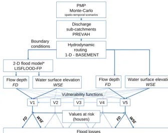
The coupled simulations of the 150 rainfall patterns provide the basis for the inundation modelling. The 1-D hydrody-namic model routes the water flow from the sub-catchments towards the catchment outlet. We defined the coupling points between the hydrological and the hydraulic model with a bottom-up approach: first, we delimited the floodplains for which the flood loss estimation will be valid (system de-limitation). Second, we defined the upper boundary condi-tions of these floodplains. Third, we delimited the upstream catchments for the hydrological model based on the coupling points. However, the location of the gauging stations was also considered in the definition of the coupling points in order to calibrate and validate the hydrological model. The 1-D hydrodynamic model computes the level of the lakes and the outflow from the lakes. However, we used a 2-D in-undation model as reference model for estimating the flow depths in the floodplains required for flood loss analysis. We nested the 2-D inundation models into the 1-D hydrodynamic model (see schematic of the approach in Fig. 1) to avoid the computationally demanding simulation of the lake retention with the 2-D model. We simulated all scenarios with the 1-D model and nested the 2-1-D model into the outcomes of the 1-D model at specific locations (boundary conditions). Hence, the 2-D model is always started after the simulation with the 1-D model in a cascading approach. The lake out-flow hydrographs and lake level hydrographs from the 1-D hydrodynamic model and the hydrographs computed by the hydrological model that are directly flowing into the flood-plains considered by the 2-D models were used as upper or lower boundary conditions for the 2-D flood inundation modelling. Minor tributaries are neglected as upper boundary condition. However, the outflows from their catchments are taken into account by aggregating all minor tributaries to sub-catchment level. The spatial setup of the model experiment, as well as the interfaces between the hydrological model and the floodplains modelled in 2-D, are shown in Fig. 2. In the 1-D model, the outflow from the sub-catchments is fed directly in the main river without considering flooding in the alluvial fans of the tributaries. In contrast, the outflows from the sub-catchments are fed into the 2-D model at the coupling points as shown in Fig. 2. Thus, the 2-D model considers flooding of the alluvial fans of the tributaries.
model was set up with a subgrid representation of the chan-nel and a spatial resolution on the floodplain of 50 m. The digital terrain model (DTM) was upscaled from a lidar DTM with high spatial resolution (0.5 m). The basis of this terrain data is a digital terrain model (DTM) provided by the Canton of Bern. This terrain model was created from lidar measure-ments collected in 2014 and 2015 with a resolution of about four points per m2. The lidar data were processed by the data provider to create a raster DTM with a cell size of 0.5 m. The buildings and the most important hydraulic structures in the main rivers (main bridges) were removed by this process. We corrected this raw raster model by (a) manually elimi-nating the remaining hydraulic obstacles in the river reaches, (b) correcting the height of the riverbanks in the Aare and Gürbe rivers reaches on the basis of DGPS measurements along the riverbanks, and (c) interpolating the altitudes of the raster cells of the river bed on the basis of surveyed bathy-metric cross sections provided by the Federal Office for the Environment (BAFU). The result is a DTM with a spatial res-olution of 0.5 m and the above mentioned corrections. This hydraulically correct DTM provides the basis for the aggre-gation at coarser spatial resolution for the flood inundation models.
The subgrid channel module requires the heights of the river bed and of the lateral dams, the river width, and the shape of the river bed. These data were computed at high resolution and aggregated onto the target resolution of the inundation model by conserving the cross-sectional area of the river channel from the high-resolution terrain model.
The 2-D hydrodynamic model was calibrated in terms of reproducing the stage–discharge relationships at the gaug-ing stations and the known channel capacity along the river reaches. The model was validated on the basis of documented flooding. The fit of the inundation model (after Bates and de Roo, 2000) computed on the basis of observed discharges of the flood event in August 2005 and a comparison between modelled and observed inundation extents ranges between 0.5 and 0.9, depending on the floodplain. The lower values can be explained by dam breaks that occurred in reality but are not considered in the model, or by recent changes in the river geometry since the last flood event (implementation of new flood defence measures).
In addition to the 2-D inundation model, we elaborated in-undation maps from the 1-D hydrodynamic simulations. We constructed water surface elevation (WSE) maps by interpo-lating the WSE values at the cross sections of the 1-D model. The projection of these WSE maps onto the digital terrain model (spatial resolution of 10 m) and the comparison with the DTM subsequently lead to a map of flow depths. 2.3 Flood loss modelling
In this study, we focused on structural damage to buildings (residential, public, and industrial buildings) without consid-ering losses to mobile assets, building contents, and
infras-tructure. The flood loss module of this model chain consists of a dataset of buildings similar to that described in Röthlis-berger et al. (2017) and Fuchs et al. (2015). Each building is represented by a polygon and is classified by type, function-ality, construction period, volume, reconstruction costs, and number of residents. Furthermore, we delineated the height of the ground floor above sea level of each building on the basis of a lidar terrain model with sub-metre resolution.
The resulting flow depths (FDs) and WSEs from the hy-drodynamic module were attributed to each building (ex-posure analysis) and used for deriving the object-specific degree of loss from the vulnerability functions and conse-quently for the estimation of object-specific losses. The flow depth was attributed to the building following two different approaches. The first approach is a direct attribution of the flow depth from the FD maps to each building. The second approach is an indirect attribution where the flow depth at each building results from the difference between the WSE raster of the flood simulation and the minimum ground floor level of the building. The idea behind this approach is to take into account local small-scale elevations of the houses. If a building footprint covers more than one cell, we used the maximum flow depth of all relevant cells of the inundation map (Bermúdez and Zischg, 2018).The flow depth was used to calculate the degree of loss on the basis of a vulnerabil-ity function. The degree of loss resulting from the flow depth and the vulnerability function was subsequently multiplied with the reconstruction value of the building. This results in the expected loss to the building structure. The object-specific losses were subsequently summed to give the cumu-lative losses of a simulated precipitation scenario.
Five vulnerability functions were considered in the damage calculation procedure. We used the functions of Totschnig et al. (2011; V1), Papathoma-Köhle et al. (2015; V2), Hydrotec (2001; V3) as cited in Merz and Thieken (2009), Jonkman et al. (2008; V4), and Dutta et al. (2003; V5). We used different vulnerability functions because there is no regionally adopted and validated vulnerability function available for Switzerland, and because we aimed explicitly at exploring the range of uncertainties related to the choice of the function and its relevance for the maximum uncer-tainties in the outcomes. A direct validation of the vulner-ability functions was not possible because of a lack of loss data at the level of single objects due to privacy restrictions. The selected vulnerability functions consider flow depths as the only input variable for the estimation of the degree of loss. We did not consider flow velocity because the inunda-tion models used in this study do not provide flow velocities and we wanted to use comparable loss models.
2.4 Benchmarking against other selected uncertainty factors
PMP Monte-Carlo spatio-temporal scenarios
Discharge sub-catchments
PREVAH Hydrodynamic
routing 1-D - BASEMENT 2-D flood model*
LISFLOOD-FP
Flood losses Values at risk
(houses)
*benchmark inundation model
V1 V2 V3 V4 V5
Vulnerability functions Boundary
conditions
Flow depth FD
Water surface elevation WSE Flow depth
FD
Water surface elevation WSE
[image:6.612.130.465.67.333.2]FD WSE FD WSE
Figure 1.Schematic of the nesting approach. The 2-D flood inundation models and the loss models are nested in a 1-D routing model.
uncertainty factors. The comparison was made by follow-ing the parallel models approach first presented by Visser et al. (2000) for the example of climate simulations. Merz and Thieken (2009) adopted this approach for the identification of principal uncertainty sources in flood risk calculations. In summary, this approach computes a number of model runs with varying input parameters. In the first step, the mini-mum and maximini-mum values of all simulation outcomes (flood losses in financial units in this study) were extracted. The difference between both is defined as the maximum uncer-tainty range (MUR). In the second step, the unceruncer-tainty range (URsub) of a specific subset of model runs was computed.
The subsets from all model runs can be defined by specific criteria, e.g. a subset of all model runs with the same flood model or a subset of model runs using the same vulnerabil-ity function. The uncertainty range of this subset is given by the difference between the minimum and maximum values of all simulation outcomes of this specific subset. Third, the reduced uncertainty range (RUR) was computed according to Eq. (1). This indicator describes the relative role of an uncer-tainty source to the maximum unceruncer-tainty range of all model runs.
RUR=(MUR−URsub)
MUR ·100 % (1)
The RUR is related to the maximum uncertainty range of all models but is not relative to the RUR of other subsets. Fur-thermore, Eq. (1) does not isolate all the contributions of the
3 Study area
We set up the flood inundation models for the main valley of the Aare River basin upstream of Bern, Switzerland. The catchment elevation ranges from 500 to 4200 m a.s.l., with a mean elevation of 1600 m a.s.l. The southern part of the river basin consists of relatively high alpine mountains. Sev-eral alpine peaks within this area exceed 4000 m a.s.l., and parts of it are glaciated (8 % of the total catchment area). The main valley of the Aare River basin consists of a relatively flat floodplain with two lakes, where widespread flooding can occur. The lakes are natural but artificially managed, and are oriented along an approximately east–west axis in the low-land part of the catchment. The study area covers 3000 km2, and the following main river reaches are considered in the model chain (see Fig. 2):
1. Hasliaare river, from Meiringen to Lake Brienz (flood-plain: 15 km2; contributing area: 451 km2);
2. Lake Brienz static inundation model (lake area: 31 km2; contributing area: 1138 km2);
3. Interlaken, area between Lake Brienz and Lake Thun and the fan of the Lütschine River (floodplain: 28 km2); 4. Lake Thun static inundation model (lake area: 50 km2;
contributing area: 2450 km2); 5. Thun (floodplain: 8 km2);
6. Aare River reach between Thun and Bern (floodplain: 42 km2);
7. Gürbe River reach between Burgistein and Belp (flood-plain: 15 km2; contributing area: 116 km2).
4 Results
The main results of the coupled model simulations are the discharges at the outlet of each of the sub-catchments, the discharge at the outlet of the Aare River basin at Bern, and the flood losses for 150 PMP simulations. Figure 3 shows the hydrographs of the 150 PMP scenarios at the outlet of the river basin in Bern. The outflow from the river basin varies remarkably in peak discharge and time to peak. The peak dis-charges for each ensemble member were in the range 906 to 1296 m3s−1. Thus, the highest peak discharge is 43 % higher than the lowest in the selected set of scenarios. Moreover, Fig. 3 shows the discharges of the tributaries downstream of Lake Thun during peak flow of the Aare River at Bern. It is shown that the highest peak discharge at Bern depends on both a high flow in the main river and high flows in the tribu-taries. Upstream of Thun, the synchronization of flood peaks is represented by the lake levels.
The flood inundation modelling resulted in a set of flood maps representing the 150 PMP scenarios. The overlay of
# # #
# # #
# # #
#
#
# #
# #
# #
# # #
# #
# # #
# # #
!Bern
0 5 10 20km
! !
IT FR
CH DE
AT LI
lake Thun lake Bri enz (6) A
are (7) G
ürbe
(1) Hasliaare (2) Lak
e
Brienz (3) Interlake
n (4) Lake
Thun
[image:7.612.313.546.65.251.2](5) Thun
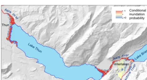
Figure 2.The Aare River catchment upstream of Bern, Switzerland. The sub-catchments of the hydrological model are divided by black lines. The black triangles indicate the coupling points between the hydrologic and the 2-D inundation model. The 1-D routing model covers all floodplains (red lines) and the lakes (blue). The flood-plains that are covered by the individual 2-D inundation models nested into the 1-D routing model are marked and labelled in red.
these flood maps leads to an inundation extent map that esti-mates a spatial probability of inundation, conditional on the rainfall sum of a PMP event in the river basin. Each inunda-tion map is treated as equally weighted in the probabilistic map. This map represents the probability that a model grid cell is flooded in one PMP scenarios. An extract of this map is shown in Fig. 4. The map shows that not all of the PMP scenarios lead to flooding of the same areas. Thus, despite the narrow framing of floodplains in mountainous areas by topography, high variability in flood extent can be observed. The discharge in the Lütschine River at Interlaken and the lake levels of both lakes, Lake Brienz and Lake Thun, have the strongest influence on the inundation probability map. In particular, the level of Lake Thun and the flooding by the Lütschine River determine a remarkable portion of the flooded area.
0 24 48 72 96 120 144 Time [h] 200
400 600 800 1000 1200 1400
Q
[
m
3s 1]
(a) Aare river at Bern
0 20 40 60 80 100 120 140
200 400 600 800 1000 1200
1400 (b) Contribution of tributaries to peak discharge
Aare Thun Zulg Rotache
Chiese Guerbe
Other
Scenario
Figure 3. (a)Hydrographs at the outlet of the Aare River basin in Bern resulting from the coupled hydrologic-hydrodynamic modelling of
the 150 PMP scenarios.(b)Superimposition of the tributaries downstream of Lake Thun during peak flow of the Aare River at Bern.
0 1 2 4 6km
Lake Thun
Lake B rienz
Aarer iver
Interlaken Thun
Lüts
chine rive
r Aare
r iver Conditionalinundation
probability 1
[image:8.612.108.494.71.226.2]>0
Figure 4.Detailed example of the conditional probability flood map for the floodplains of Thun and Interlaken. Predicted flood inunda-tion extents can change significantly depending on the specific spa-tial properties of a few of the PMP scenarios and hence have lower mapped inundation probabilities.
only considers flooding by the main river Aare and neglects the tributaries.
The flood simulation mapped outputs (flow depth maps and water surface elevation maps) were used separately to calculate the flood losses at the individual building level. Subsequently, the flood losses at building scale were aggre-gated at a catchment level. Figure 6 shows the distribution of the aggregated flood losses. It is shown that – depending on the model ensemble member – the losses vary between CHF 0.06 and 2.87 billion. Thus, the losses are remarkably influenced by all the experimental uncertainty factors pre-viously discussed in the modelling chain. However, even if the effect of the vulnerability function and the choice of the exposure analysis approach are not considered, the losses still vary markedly depending on the PMP scenario. Maxi-mum losses are still approximately 3–5 times the miniMaxi-mum losses for some of the vulnerability functions. The vulnera-bility function V4 (Jonkman et al., 2008) results in the lowest
losses. This function was calibrated for lowland floodplains and thus has generally lower degrees of loss. However, this vulnerability function might be more representative for the areas affected by lake flooding than the others. In the 2-D FD model runs, the exposure is higher compared to the 2-D WSE model runs. In contrast, the losses are higher in the 2-D WSE run. This relates to the mean flow depths at the buildings. The mean flow depth over all affected buildings is 0.54 m in the 2-D FD model runs and 0.87 m in the 2-D WSE model runs. This results in higher losses although the number of exposed buildings is lower. The flow depths in the 1-D FD and 1-D WSE model runs are 1.08 and 1.36 m respectively. This explains the generally higher losses in the 1-D model runs compared to the 2-D model runs.
The benchmark against other uncertainties such as the flood modelling in combination with the exposure analy-sis approach and the vulnerability functions shows that the uncertainties considered in the model experiment contribute significantly to the sensitivity of the model chain to the as-sumptions made. Each member of the ensemble runs repre-sents a rainfall pattern and a resulting flood loss computed on a basis of a combination of a specific flood model with a specific loss model. The difference between the ensemble member with the absolute minimum and the member with the absolute maximum of flood losses represents the maxi-mum uncertainty range MUR. The total number of runs was divided into subsets that represents in each case the uncer-tainty range of a specific combination of the variables. The difference between the member with the absolute minimum of this subset and the member with the absolute maximum of this subset represents the reduced uncertainty range URsub.
[image:8.612.49.286.286.416.2]vari-2-D FD 2-D WSE 1-D FD 1-D WSE 2500
3000 3500 4000 4500 5000 5500
2-D FD 2-D WSE 1-D FD 1-D WSE
10 000 12 000 14 000 16 000 18 000 20 000 22 000 24 000 26 000
Exposed buildings
(a) Exposed buildings
Exposed residents
[image:9.612.120.477.70.225.2](b) Exposed residents
Figure 5.Exposed buildings(a)and residents(b)aggregated at river basin level. Flood losses aggregated at river basin level. The variation
between the PMP scenarios is shown on theyaxis, whereas thexaxis shows the variability inherent to the choice of the flood model
(2-D: LISFLOOD-FP; 1-(2-D: BASEMENT-1D) in combination with the approach for attributing flow depths to the buildings (F(2-D: flow depths are calculated on the basis of flow depths maps; WSE: flow depths are calculated on the basis of water surface elevation maps and the object-specific ground floor level).
ability in rainfall scenarios lies between 42 and 92 % with a median of 72 %. Hence, the highest RUR of all subsets is dominated by the subsets regarding the variability in proba-ble maximum precipitation pattern. Figure 7 shows the com-parison between the RUR values of the subsets in which the variability of one of the three considered uncertainty factors was analysed. This analysis makes evident that the rainfall pattern contributes most to the maximum uncertainty range.
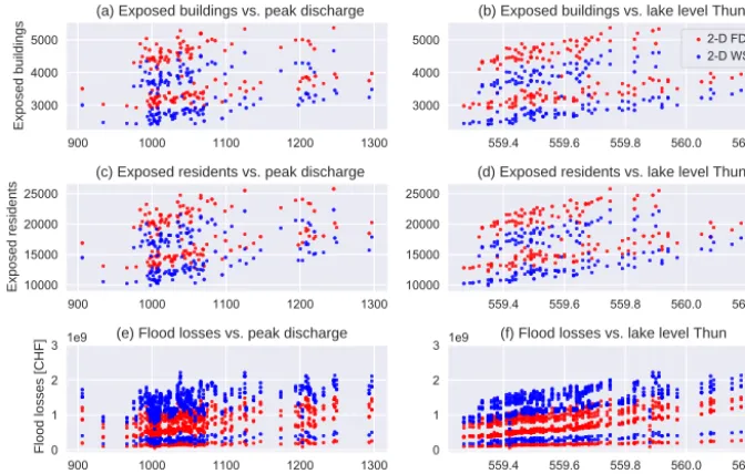
In Fig. 8 (left column), we plotted the results of all model outcomes with focus on the 2-D inundation model in terms of exposed number of buildings and persons, and in terms of flood losses against the peak discharge of the respective precipitation pattern at the catchment outlet. The hypothesis that the flood losses increase with peak discharge at the out-let of the river basin can be verified in the sense that there is a significant correlation. This relationship is weaker for exposed buildings and residents than for the flood losses. However, the rainfall scenario leading to the highest peak discharge at the basin outlet does not correspond with the highest flood losses. Instead, the flood losses are more cor-related with high lake levels in Lake Thun (see Fig. 8, right column). The correlation between flood losses and the level of Lake Thun (Spearman’s rank correlation coefficient ranges from 0.54 to 0.94, depending on the flood model and the vul-nerability function) is stronger than between losses and the peak discharge at the catchment outlet (Spearman’s rank cor-relation coefficient ranging from 0.43 to 0.71). Thus, in the Aare River basin, the level of Lake Thun is a more relevant proxy indicator for the amount of flood losses in the whole river basin than the peak discharge at the outlet of the river basin (i.e. the so-called PMF of the river basin). This can be explained by the local situation of the city of Thun where the density of the building stock is very high along the shore-line of Lake Thun and along the Aare River. The major area
of the Aare River basin contributes to the lakes. Only 20 % of the catchment area is located downstream of Lake Thun. Although the area of Lake Thun covers only about 2 % of its contributing area, this means that the river basin has rele-vant retention areas that attenuate the outflow from the river basin and thus the PMF. Vice versa, this retention effect in-creases flood losses because a relevant number of buildings are located in neighbourhood of the lake shorelines. Like-wise, not all of the PMP scenarios lead to flooding by the Lütschine River in Interlaken. As shown in Fig. 4, the flood-plain of this river is flooded only in a minority of the ensem-ble runs. Depending on whether this floodplain is flooded or not, up to 1500 exposed buildings and therefore up to one-third of the total number of maximally exposed buildings in the whole river basin could be affected. Thus, the highest loss of all simulated scenarios is related to a combination of a high lake level in Thun with high river discharge of the Lütschine River. This shows that the maximum loss depends on both the spatio-temporal pattern of the rainfall and the in-ternal organization of the river basin in terms of the spatial distribution of the values at risk (i.e. exposure) within the floodplains.
5 Discussion and conclusions
Further-V1 V2 V3 V4 V5 0.0
0.6 1.2 1.8 2.4 3.0
Flood losses [CHF]
1e9 (a) LISFLOOD-FP FD
V1 V2 V3 V4 V5
0.0 0.6 1.2 1.8 2.4
3.0 1e9 (b) LISFLOOD-FP WSE
V1 V2 V3 V4 V5
Vulnerability function 0.0
0.6 1.2 1.8 2.4 3.0
Flood losses [CHF]
1e9 (c) 1-D FD
V1 V2 V3 V4 V5
Vulnerability function 0.0
0.6 1.2 1.8 2.4 3.0 1e9
[image:10.612.132.465.68.317.2](d) 1-D WSE
Figure 6.Flood losses aggregated at river basin level. The variation between the PMP scenarios is shown in theyaxis, whereas thexaxis
shows the variability inherent to the vulnerability functions. The diagram in(a)shows flood losses that are calculated based on the flow
depths as modelled by LISFLOOD-FP, the diagram in(b)shows the flood losses that are calculated based on the water surface elevation and
the object-specific ground floor level. The flood losses estimated by the 1-D model are shown in(c)and(d).
RUR precipitation RUR floodmodel RUR vulnerability 0
20 40 60 80 100
Contribution to uncertainty range [%]
Figure 7.Reduced uncertainty ranges RUR of the subsets of model runs representing the three main uncertainty sources.
more, we benchmarked these effects with other uncertainties in flood loss modelling.
The model experiment showed that the sensitivity of flood losses to the variability of spatial distribution of rainfall within a river basin with a complex topography is larger than for the other considered uncertainty factors. The PMP pattern determines the magnitude and timing of the flood peaks com-ing from the sub-catchments and flowcom-ing through the flood-plains along the main valleys and the lakes. Thus, the rainfall
pattern could lead to a superimposition of flood waves as de-scribed by the model experiments of Neal et al. (2013) and Pattison et al. (2014). In addition to the superimposition of flood waves, it is shown that lake levels, as a proxy for the water volumes coming from different sub-catchments, are also relevant for the determination of flood losses. This com-plements the findings of Sampson et al. (2014) on the im-pacts of precipitation variability on insurance loss estimates. With the present study, we extended the Sampson et al. study, which was focussed on urban environments, with a focus on complex mountainous river basins.
[image:10.612.54.278.401.551.2]900 1000 1100 1200 1300 3000
4000 5000
Exposed buildings
(a) Exposed buildings vs. peak discharge
559.4 559.6 559.8 560.0 560.2 3000
4000 5000
(b) Exposed buildings vs. lake level Thun
2-D FD 2-D WSE
900 1000 1100 1200 1300
10000 15000 20000 25000
Exposed residents
(c) Exposed residents vs. peak discharge
559.4 559.6 559.8 560.0 560.2 10000
15000 20000 25000
(d) Exposed residents vs. lake level Thun
900 1000 1100 1200 1300
Qpeak [m3s1] 0
1 2 3
Flood losses [CHF]
1e9 (e) Flood losses vs. peak discharge
559.4 559.6 559.8 560.0 560.2
Lake level Thun [m a.s.l.]
0 1 2
[image:11.612.130.466.71.285.2]3 1e9 (f) Flood losses vs. lake level Thun
Figure 8.This figure shows the aggregated flood losses for the 150 PMP scenarios. The red dots show the exposed entities and losses that are computed based on the flow depths, the blue dots show the exposed entities and losses that are computed based on water surface elevation. The figures in the last row show the losses resulting from all vulnerability functions.
the variability in rainfall pattern lead to a specific sensitivity of the whole river basin to a certain pattern of rainfall. This behaviour has to be analysed and generalized in further stud-ies and considered in the estimation of probable maximum flood losses.
Despite the topographical confinement of the floodplains by the mountain hillslopes, the flooded areas vary markedly with different rainfall patterns. Thus, the probabilistic map shows high spatial variability, caused by a few of the PMP scenarios significantly increasing inundation areas. Hence, the flow depths even at the individual building level, and con-sequently the total flood losses, vary remarkably with rainfall scenario. This case study in a mountainous environment and in an environment with remarkable retention capacities due to the presence of lakes may even lead to an attenuated il-lustration of this effect. These retention effects attenuate the PMF on one side but control the flood losses on the other side if settlements are located alongside the lakes. However, in mountain areas without lakes, the effects of spatio-temporal variability in precipitation patterns on flood losses may be even more accentuated. However, a modelling approach is needed to analyse these effects as stated by Emmanuel et al. (2015).
Nevertheless, the other uncertainty factors considered in this study, i.e. the role of the flood model, the exposure as-sessment approach and the vulnerability functions, are also contributing markedly to the maximum uncertainty range. This is in line with the findings of other studies (Jongman et al., 2012; de Moel and Aerts, 2011). Consequently, these
uncertainties also have to be taken into account in portfolio analysis or in the analysis of probable maximum flood losses. In summary, we conclude that the analysis of a broader set of extreme floods with different precipitation patterns leads to more a comprehensive view of flood losses in a river basin compared to standard deterministic PMP/PMF methods. The spatio-temporal characteristics of rainfall patterns must be considered in complex mountainous river basins. Moreover, the analysis of the probable maximum flood losses in a river basin should consider the systemic vulnerability of the flood-plains or the behaviour of floodflood-plains as human–water sys-tems as stated by Di Baldassarre et al. (2013, 2014). This involves the identification of key locations of exposure that contribute most to the overall flood losses. Probabilistic in-undation maps provide a first overview of key locations of flooded areas with high sensitivity against the rainfall pat-tern. Furthermore, it is shown that the presented model ex-periment provides a valuable instrument for the considera-tion of all components in the analysis of the variability of rainfall patterns to flood losses in a river basin, from hazard to exposure to vulnerability.
basis of the system characteristics of the river basin (sensi-tivities of floodplains and spatial setup of the river system). The calculation of the maximum expectable flood losses in a river basin should not be based exclusively on the PMF. In contrast to the initial hypothesis, we observed that other catchment characteristics in combination with the PMF could remarkably influence the flood losses. Consequently, in com-plex river basins it is recommended to analyse the sensitivity of the most relevant floodplains before analysing the proba-ble maximum flood losses.
Code availability. Data of cross section surveys were provided the Federal Office for the Environment. The lidar terrain model was provided by the Canton of Bern. Basic GIS data were provided by the Federal Office for Topography swisstopo. The residential regis-ter was provided by the Federal Office for Statistics. The data about values at risk are restricted by privacy regulations. All other data produced in this study and the codes for the model experiment are available from the leading author on request. The inundation model LISFLOOD-FP is available at http://www.bristol.ac.uk/geography/ research/hydrology/models/lisflood/ (Bates, 2018).
Author contributions. The study was designed by APZ, JF, PB, and RW. The hydrological model was set up and run by GF. Model cou-pling and the set up of the hydraulic model were done by APZ, NQ, GC, and JN. The loss model was developed by APZ. The analy-ses were performed by APZ with the support of all co-authors. The manuscript was prepared by APZ with the contribution of all co-authors.
Competing interests. The authors declare that they have no conflict of interest.
Acknowledgements. The work was partially funded by the Swiss National Foundation (grant no. IZK0Z2_170478/1), by the Swiss Mobiliar, by NERC grant SINATRA (Susceptibility of catchments to INTense RAinfall and flooding, grant no. NE/K008781/1), and by NERC grant MaRIUS (Managing the Risks, Impacts and Uncer-tainties of droughts and water Scarcity, grant no. NE/L010399/1). We thank the Federal Government of Switzerland and the Canton of Bern for providing the data.
Edited by: Erwin Zehe
Reviewed by: two anonymous referees
References
Adams, R., Western, A. W., and Seed, A. W.: An analysis of the impact of spatial variability in rainfall on runoff and sediment predictions from a distributed model, Hydrol. Process., 26, 3263– 3280, https://doi.org/10.1002/hyp.8435, 2012.
Altarejos-García, L., Martínez-Chenoll, M. L., Escuder-Bueno, I., and Serrano-Lombillo, A.: Assessing the impact of uncertainty
on flood risk estimates with reliability analysis using 1-D and 2-D hydraulic models, Hydrol. Earth Syst. Sci., 16, 1895–1914, https://doi.org/10.5194/hess-16-1895-2012, 2012.
Apel, H., Merz, B., and Thieken, A. H.: Quantification of uncer-tainties in flood risk assessments, Int. J. River Basin Manage., 6, 149–162, https://doi.org/10.1080/15715124.2008.9635344, 2008.
Arnell, N. W. and Gosling, S. N.: The impacts of climate change on river flood risk at the global scale, Clim. Change, 134, 387–401, https://doi.org/10.1007/s10584-014-1084-5, 2016.
Asadieh, B. and Krakauer, N. Y.: Global trends in extreme pre-cipitation: climate models versus observations, Hydrol. Earth Syst. Sci., 19, 877–891, https://doi.org/10.5194/hess-19-877-2015, 2015.
Bates, P.: LISFLOOD-FP. Model description and download, avail-able at: http://www.bristol.ac.uk/geography/research/hydrology/ models/lisflood/, last access: 4 May 2018.
Bates, P. D. and de Roo, A. P. J.: A simple raster-based model for flood inundation simulation, J. Hydrol., 236, 54–77, https://doi.org/10.1016/S0022-1694(00)00278-X, 2000. Bates, P. D., Horritt, M. S., and Fewtrell, T. J.: A simple inertial
formulation of the shallow water equations for efficient two-dimensional flood inundation modelling, J. Hydrol., 387, 33–45, https://doi.org/10.1016/j.jhydrol.2010.03.027, 2010.
Beauchamp, J., Leconte, R., Trudel, M., and Brissette, F.: Estima-tion of the summer-fall PMP and PMF of a northern watershed under a changed climate, Water Resour. Res., 49, 3852–3862, https://doi.org/10.1002/wrcr.20336, 2013.
Beniston, M., Stephenson, D. B., Christensen, O. B., Ferro, C. A. T., Frei, C., Goyette, S., Halsnaes, K., Holt, T., Jylhä, K., Koffi, B., Palutikof, J., Schöll, R., Semmler, T., and Woth, K.: Future extreme events in European climate: An exploration of regional climate model projections, Clim. Change, 81, 71–95, https://doi.org/10.1007/s10584-006-9226-z, 2007.
Bermúdez, M. and Zischg, A. P.: Sensitivity of flood loss es-timates to building representation and flow depth attribution methods in micro-scale flood modelling, Nat. Hazards, 14, 253, https://doi.org/10.1007/s11069-018-3270-7, 2018.
Bouwer, L. M.: Projections of future extreme weather losses un-der changes in climate and exposure, Risk analysis an offi-cial publication of the Society for Risk Analysis, 33, 915–930, https://doi.org/10.1111/j.1539-6924.2012.01880.x, 2013. Bruni, G., Reinoso, R., van de Giesen, N. C., Clemens, F. H. L. R.,
and ten Veldhuis, J. A. E.: On the sensitivity of urban hydrody-namic modelling to rainfall spatial and temporal resolution, Hy-drol. Earth Syst. Sci., 19, 691–709, https://doi.org/10.5194/hess-19-691-2015, 2015.
Büchele, B., Kreibich, H., Kron, A., Thieken, A., Ihringer, J., Oberle, P., Merz, B., and Nestmann, F.: Flood-risk mapping: contributions towards an enhanced assessment of extreme events and associated risks, Nat. Hazards Earth Syst. Sci., 6, 485–503, https://doi.org/10.5194/nhess-6-485-2006, 2006.
Burke, N., Rau-Chaplin, A., and Varghese, B.: Computing probable maximum loss in catastrophe reinsurance portfolios on multi-core and many-multi-core architectures, Concurrency Computat.: Pract. Exper., 28, 836–847, https://doi.org/10.1002/cpe.3695, 2016.
with emergency storage areas, Hydrol. Process., 22, 4695–4709, https://doi.org/10.1002/hyp.7079, 2008.
Coxon, G., Freer, J., Westerberg, I. K., Wagener, T., Woods, R., and Smith, P. J.: A novel framework for discharge uncertainty quantification applied to 500 UK gauging stations, Water Resour. Res., 51, 5531–5546, https://doi.org/10.1002/2014WR016532, 2015.
Cristiano, E., ten Veldhuis, M.-C., and van de Giesen, N.: Spatial and temporal variability of rainfall and their effects on hydro-logical response in urban areas – a review, Hydrol. Earth Syst. Sci., 21, 3859–3878, https://doi.org/10.5194/hess-21-3859-2017, 2017.
de Moel, H. and Aerts, J. C. J. H.: Effect of uncertainty in land use, damage models and inundation depth on flood damage estimates, Nat. Hazards, 58, 407–425, https://doi.org/10.1007/s11069-010-9675-6, 2011.
de Moel, H., Jongman, B., Kreibich, H., Merz, B., Penning-Rowsell, E., and Ward, P. J.: Flood risk assessments at different spatial scales, Mitig. Adapt. Strateg. Glob. Change, 20, 865–890, https://doi.org/10.1007/s11027-015-9654-z, 2015.
Di Baldassarre, G., Schumann, G., Bates, P. D., Freer, J. E., and Beven, K. J.: Flood-plain mapping: A critical discussion of de-terministic and probabilistic approaches, Hydrol. Sci. J., 55, 364– 376, https://doi.org/10.1080/02626661003683389, 2010. Di Baldassarre, G., Kooy, M., Kemerink, J. S., and Brandimarte, L.:
Towards understanding the dynamic behaviour of floodplains as human-water systems, Hydrol. Earth Syst. Sci., 17, 3235–3244, https://doi.org/10.5194/hess-17-3235-2013, 2013.
Di Baldassarre, G., Kemerink, J. S., Kooy, M., and Brandimarte, L.: Floods and societies: the spatial distribution of water-related disaster risk and its dynamics, WIREs Water, 1, 133–139, https://doi.org/10.1002/wat2.1015, 2014.
Dodov, B. and Foufoula-Georgiou, E.: Incorporating the spatio-temporal distribution of rainfall and basin geomorphology into nonlinear analyses of streamflow dynamics, Adv. Water Resour., 28, 711–728, https://doi.org/10.1016/j.advwatres.2004.12.013, 2005.
Dutta, D., Herath, S., and Musiake, K.: A mathematical model for flood loss estimation, J. Hydrol., 277, 24–49, https://doi.org/10.1016/S0022-1694(03)00084-2, 2003. Emmanuel, I., Andrieu, H., Leblois, E., Janey, N., and Payrastre, O.:
Influence of rainfall spatial variability on rainfall–runoff mod-elling: Benefit of a simulation approach?, J. Hydrol., 531, 337– 348, https://doi.org/10.1016/j.jhydrol.2015.04.058, 2015. Emmanuel, I., Payrastre, O., Andrieu, H., Zuber, F., Lang, M.,
Klijn, F., and Samuels, P.: Influence of the spatial variability of rainfall on hydrograph modelling at catchment outlet: A case study in the Cevennes region, France, E3S Web Conf., 7, 18004, https://doi.org/10.1051/e3sconf/20160718004, 2016.
Faulkner, D. and Benn, J.: Reservoir Flood Estimation: Time for a Re-think, in: Dams – Benefits and Disbenefits; Assets or Liabili-ties?, edited by: Pepper, A., ICE Publishing, London, 2016.
Felder, G. and Weingartner, R.: An approach for the
determination of precipitation input for worst-case
flood modelling, Hydrol. Sci. J., 61, 2600–2609,
https://doi.org/10.1080/02626667.2016.1151980, 2016. Felder, G. and Weingartner, R.: Assessment of deterministic
PMF modelling approaches, Hydrol. Sci. J., 62, 1591–1602, https://doi.org/10.1080/02626667.2017.1319065, 2017.
Felder, G., Zischg, A., and Weingartner, R.: The effect of coupling hydrologic and hydrodynamic models on proba-ble maximum flood estimation, J. Hydrol., 550, 157–165, https://doi.org/10.1016/j.jhydrol.2017.04.052, 2017.
Fewtrell, T. J., Bates, P. D., Horritt, M., and Hunter, N. M.: Evaluating the effect of scale in flood inundation modelling in urban environments, Hydrol. Process., 22, 5107–5118, https://doi.org/10.1002/hyp.7148, 2008.
Fischer, E. M. and Knutti, R.: Observed heavy precipitation increase confirms theory and early models, Nat. Clim. Change, 6, 986– 991, https://doi.org/10.1038/nclimate3110, 2016.
Foufoula-Georgiou, E.: A probabilistic storm transposition
approach for estimating exceedance probabilities of ex-treme precipitation depths, Water Resour. Res., 25, 799–815, https://doi.org/10.1029/WR025i005p00799, 1989.
Franchini, M., Helmlinger, K. R., Foufoula-Georgiou, E., and Todini, E.: Stochastic storm transposition coupled with
rainfall–runoff modeling for estimation of exceedance
probabilities of design floods, J. Hydrol., 175, 511–532, https://doi.org/10.1016/S0022-1694(96)80022-9, 1996.
Fuchs, S., Keiler, M., and Zischg, A.: A
spatiotempo-ral multi-hazard exposure assessment based on
prop-erty data, Nat. Hazards Earth Syst. Sci., 15, 2127–2142, https://doi.org/10.5194/nhess-15-2127-2015, 2015.
Gai, L., Baartman, J. E. M., Mendoza-Carranza, M., Wang, F., Ritsema, C. J., and Geissen, V.: A framework ap-proach for unravelling the impact of multiple factors influ-encing flooding, J. Flood Risk Manage, published online first, https://doi.org/10.1111/jfr3.12310, 2017.
Gupta, H. V., Kling, H., Yilmaz, K. K., and Martinez, G. F.: Decomposition of the mean squared error and NSE performance criteria: Implications for improving hydrolog-ical modelling, Hydrology Conference 2010, 377, 80–91, https://doi.org/10.1016/j.jhydrol.2009.08.003, 2009.
Hasan, S. and Foliente, G.: Modeling infrastructure system inter-dependencies and socioeconomic impacts of failure in extreme events: emerging R&D challenges, Nat. Hazards, 78, 2143–2168, https://doi.org/10.1007/s11069-015-1814-7, 2015.
Horritt, M. S. and Bates, P. D.: Effects of spatial resolution on a raster based model of flood flow, J. Hydrol., 253, 239–249, https://doi.org/10.1016/S0022-1694(01)00490-5, 2001. Horritt, M. S. and Bates, P. D.: Evaluation of 1D and 2D numerical
models for predicting river flood inundation, J. Hydrol., 268, 87– 99, https://doi.org/10.1016/S0022-1694(02)00121-X, 2002. Hydrotec: Hochwasser-Aktionsplan Angerbach, Teil I: Berichte
und Anlagen, Studie im Auftrag des Stua Dusseldorf, Aachen, Germany, 2001.
IPCC: Managing the risks of extreme events and disasters to ad-vance climate change adaptation: Special report of the Inter-governmental Panel on Climate Change, Cambridge University Press, New York, x, 582, 2012.
Jongman, B., Kreibich, H., Apel, H., Barredo, J. I., Bates, P. D., Feyen, L., Gericke, A., Neal, J., Aerts, J. C. J. H., and Ward, P. J.: Comparative flood damage model assessment: towards a Eu-ropean approach, Nat. Hazards Earth Syst. Sci., 12, 3733–3752, https://doi.org/10.5194/nhess-12-3733-2012, 2012.
Modelling for Effective and Sustainable Water Management, 66, 77–90, https://doi.org/10.1016/j.ecolecon.2007.12.022, 2008. Kling, H., Fuchs, M., and Paulin, M.: Runoff conditions in the
upper Danube basin under an ensemble of climate change scenarios, Hydrology Conference 2010, 424–425, 264–277, https://doi.org/10.1016/j.jhydrol.2012.01.011, 2012.
Kvoˇcka, D., Falconer, R. A., and Bray, M.: Appropriate model use for predicting elevations and inundation extent for extreme flood events, Nat. Hazards, 79, 1791–1808, https://doi.org/10.1007/s11069-015-1926-0, 2015.
Lagos-Zuniga, M. A. and Vargas, M. X.: PMP and PMF
estimations in sparsely-gauged Andean basins and
cli-mate change projections, Hydrol. Sci. J., 59, 2027–2042, https://doi.org/10.1080/02626667.2013.877588, 2014.
McMillan, H., Krueger, T., and Freer, J.: Benchmarking ob-servational uncertainties for hydrology: Rainfall, river dis-charge and water quality, Hydrol. Process., 26, 4078–4111, https://doi.org/10.1002/hyp.9384, 2012.
Mechler, R., Hochrainer, S., Aaheim, A., Salen, H., and Wreford, A.: Modelling economic impacts and adapta-tion to extreme events: Insights from European case stud-ies, Mitig. Adapt. Strateg. Glob. Change, 15, 737–762, https://doi.org/10.1007/s11027-010-9249-7, 2010.
Merz, B. and Thieken, A. H.: Flood risk curves and
uncertainty bounds, Nat. Hazards, 51, 437–458,
https://doi.org/10.1007/s11069-009-9452-6, 2009.
Michaelides, S.: Vulnerability of transportation to extreme
weather and climate change, Nat. Hazards, 72, 1–4,
https://doi.org/10.1007/s11069-013-0975-5, 2014.
Micovic, Z., Schaefer, M. G., and Taylor, G. H.: Uncertainty anal-ysis for Probable Maximum Precipitation estimates, J. Hydrol.,
521, 360–373, https://doi.org/10.1016/j.jhydrol.2014.12.033,
2015.
Millán, M. M.: Extreme hydrometeorological events and cli-mate change predictions in Europe, J. Hydrol., 518, 206–224, https://doi.org/10.1016/j.jhydrol.2013.12.041, 2014.
Morrill, E. P. and Becker, J. F.: Defining and Analyzing the Fre-quency and Severity of Flood Events to Improve Risk Man-agement from a Reinsurance Standpoint, Hydrol. Earth Syst. Sci. Discuss., https://doi.org/10.5194/hess-2017-167, in review, 2017.
Nash, J. E. and Sutcliffe, J. V.: River flow forecasting through con-ceptual models part I – A discussion of principles, J. Hydrol., 10, 282–290, 1970.
Neal, J., Schumann, G., Fewtrell, T., Budimir, M., Bates, P., and Mason, D.: Evaluating a new LISFLOOD-FP formulation with data from the summer 2007 floods in Tewkesbury, UK, J. Flood Risk Manage, 4, 88–95, https://doi.org/10.1111/j.1753-318X.2011.01093.x, 2011.
Neal, J., Schumann, G., and Bates, P. D.: A subgrid channel model for simulating river hydraulics and floodplain inundation over large and data sparse areas, Water Resour. Res., 48, 1–16, https://doi.org/10.1029/2012WR012514, 2012a.
Neal, J., Villanueva, I., Wright, N., Willis, T., Fewtrell, T., and Bates, P. D.: How much physical complexity is needed to model flood inundation?, Hydrol. Process., 26, 2264–2282, https://doi.org/10.1002/hyp.8339, 2012b.
Neal, J., Keef, C., Bates, P., Beven, K., and Leedal, D.: Probabilistic flood risk mapping including spatial dependence, Hydrol. Pro-cess., 27, 1349–1363, https://doi.org/10.1002/hyp.9572, 2013. Neal, J. C., Bates, P. D., Fewtrell, T. J., Hunter, N. M., Wilson, M.
D., and Horritt, M. S.: Distributed whole city water level mea-surements from the Carlisle 2005 urban flood event and compar-ison with hydraulic model simulations, J. Hydrol., 368, 42–55, https://doi.org/10.1016/j.jhydrol.2009.01.026, 2009.
Nicótina, L., Alessi Celegon, E., Rinaldo, A., and Marani, M.: On the impact of rainfall patterns on the hydrologic response, Water Resour. Res., 44, 311, https://doi.org/10.1029/2007WR006654, 2008.
Nikolopoulos, E. I., Borga, M., Zoccatelli, D., and Anagnostou, E. N.: Catchment-scale storm velocity: Quantification, scale depen-dence and effect on flood response, Hydrol. Sci. J., 59, 1363– 1376, https://doi.org/10.1080/02626667.2014.923889, 2014. Ochoa-Rodriguez, S., Wang, L.-P., Gires, A., Pina, R. D.,
Reinoso-Rondinel, R., Bruni, G., Ichiba, A., Gaitan, S., Cristiano, E., van Assel, J., Kroll, S., Murlà-Tuyls, D., Tisserand, B., Schertzer, D., Tchiguirinskaia, I., Onof, C., Willems, P., and ten Veldhuis, M.-C.: Impact of spatial and temporal resolu-tion of rainfall inputs on urban hydrodynamic modelling out-puts: A multi-catchment investigation, J. Hydrol., 531, 389–407, https://doi.org/10.1016/j.jhydrol.2015.05.035, 2015.
Papathoma-Köhle, M., Zischg, A., Fuchs, S., Glade, T., and Keiler, M.: Loss estimation for landslides in mountain ar-eas – An integrated toolbox for vulnerability assessment and damage documentation, Environ. Modell. Softw., 63, 156–169, https://doi.org/10.1016/j.envsoft.2014.10.003, 2015.
Paschalis, A., Fatichi, S., Molnar, P., Rimkus, S., and Burlando, P.: On the effects of small scale space?: Time variability of rainfall on basin flood response, J. Hydrology, 514, 313–327, https://doi.org/10.1016/j.jhydrol.2014.04.014, 2014.
Pattison, I., Lane, S. N., Hardy, R. J., and Reaney, S. M.: The role of tributary relative timing and sequencing in controlling large floods, Water Resour. Res., 5444–5458, https://doi.org/10.1002/2013WR014067, 2014.
Pfahl, S., O’Gorman, P. A., and Fischer, E. M.: Under-standing the regional pattern of projected future changes in extreme precipitation, Nat. Clim. Change, 7, 423–427, https://doi.org/10.1038/nclimate3287, 2017.
Pianosi, F., Beven, K., Freer, J., Hall, J. W., Rougier, J., Stephenson, D. B., and Wagener, T.: Sensitivity analy-sis of environmental models: A systematic review with practical workflow, Environ. Modell. Softw., 79, 214–232, https://doi.org/10.1016/j.envsoft.2016.02.008, 2016.
Rafieeinasab, A., Norouzi, A., Kim, S., Habibi, H., Nazari, B., Seo, D.-J., Lee, H., Cosgrove, B., and Cui, Z.: Toward high-resolution flash flood prediction in large urban areas – Analysis of sensitivity to spatiotemporal resolution of rain-fall input and hydrologic modeling, J. Hydrol., 531, 370–388, https://doi.org/10.1016/j.jhydrol.2015.08.045, 2015.
Rajczak, J., Pall, P., and Schär, C.: Projections of extreme precip-itation events in regional climate simulations for Europe and the Alpine Region, J. Geophys. Res.-Atmos., 118, 3610–3626, https://doi.org/10.1002/jgrd.50297, 2013.
Sci., 19, 2981–2998, https://doi.org/10.5194/hess-19-2981-2015, 2015.
Röthlisberger, V., Zischg, A. P., and Keiler, M.: Identifying spatial clusters of flood exposure to support decision mak-ing in risk management, Sci. Total Environ., 598, 593–603, https://doi.org/10.1016/j.scitotenv.2017.03.216, 2017.
Rouhani, H. and Leconte, R.: A novel method to estimate the maxi-mization ratio of the Probable Maximum Precipitation (PMP) us-ing regional climate model output, Water Resour. Res., 52, 7347– 7365, https://doi.org/10.1002/2016WR018603, 2016.
Rousseau, A. N., Klein, I. M., Freudiger, D., Gagnon, P., Frigon, A., and Ratté-Fortin, C.: Development of a methodology to evaluate probable maximum precipitation (PMP) under changing climate conditions: Application to southern Quebec, Canada, J. Hydrol., 519, 3094–3109, https://doi.org/10.1016/j.jhydrol.2014.10.053, 2014.
Saksena, S. and Merwade, V.: Incorporating the
ef-fect of DEM resolution and accuracy for improved
flood inundation mapping, J. Hydrol., 530, 180–194,
https://doi.org/10.1016/j.jhydrol.2015.09.069, 2015.
Salas, J. D., Gavilán, G., Salas, F. R., Julien, P. Y., and Abdullah, J.: Uncertainty of the PMP and PMF, in: Handbook of Engineering Hydrology, vol. 2: Modeling, Climate Change and Variability, 575–603, 2014.
Salas, J. D., Tarawneh, Z., and Biondi, F.: A hydrologi-cal record extension model for reconstructing streamflows from tree-ring chronologies, Hydrol. Process., 29, 544–556, https://doi.org/10.1002/hyp.10160, 2015.
Sampson, C. C., Fewtrell, T. J., O’Loughlin, F., Pappenberger, F., Bates, P. B., Freer, J. E., and Cloke, H. L.: The impact of un-certain precipitation data on insurance loss estimates using a flood catastrophe model, Hydrol. Earth Syst. Sci., 18, 2305– 2324, https://doi.org/10.5194/hess-18-2305-2014, 2014. Sanyal, J.: Uncertainty in levee heights and its effect on the spatial
pattern of flood hazard in a floodplain, Hydrol. Sci. J., 62, 1483– 1498, https://doi.org/10.1080/02626667.2017.1334887, 2017. Savage, J. T. S., Bates, P., Freer, J., Neal, J., and Aronica, G.:
When does spatial resolution become spurious in probabilistic flood inundation predictions?, Hydrol. Process., 30, 2014–2032, https://doi.org/10.1002/hyp.10749, 2015.
Scherrer, S. C., Fischer, E. M., Posselt, R., Liniger, M. A., Croci-Maspoli, M., and Knutti, R.: Emerging trends in heavy precipitation and hot temperature extremes in
Switzerland, J. Geophys. Res.-Atmos., 121, 2626–2637,
https://doi.org/10.1002/2015JD024634, 2016.
Singh, V. P.: Effect of spatial and temporal variability in rainfall and watershed characteristics on stream flow hydrograph, Hydrol. Process., 11, 1649–1669, https://doi.org/10.1002/(SICI)1099-1085(19971015)11:12<1649::AID-HYP495>3.0.CO;2-1, 1997. Smolka, A.: Natural disasters and the challenge of extreme events:
Risk management from an insurance perspective, Philos. T. R. Soc. A, 364, 2147–2165, https://doi.org/10.1098/rsta.2006.1818, 2006.
Stratz, S. A. and Hossain, F.: Probable Maximum Precipitation in a Changing Climate: Implications for Dam Design, J. Hydrol. Eng., 19, 6014006, https://doi.org/10.1061/(ASCE)HE.1943-5584.0001021, 2014.
Totschnig, R., Sedlacek, W., and Fuchs, S.: A quantitative vulner-ability function for fluvial sediment transport, Nat. Hazards, 58, 681–703, https://doi.org/10.1007/s11069-010-9623-5, 2011. UNISDR: Making development sustainable: The future of disaster
risk management, Global assessment report on disaster risk re-duction, 4.2015, United Nations, Geneva, 311 p., 2015. Vetsch, D., Siviglia, A., Ehrbar, D., Facchini, M., Gerber, M.,
Kam-merer, S., Peter, S., Vonwiler, L., Volz, C., Farshi, D., Mueller, R., Rousselot, P., Veprek, R., and Faeh, R.: BASEMENT – Ba-sic Simulation Environment for Computation of Environmental Flow and Natural Hazard Simulation, Zurich, 2017.
Visser, H., Folkert, R. J. M., Hoekstra, J., and de Wolff, J. J.: Identifying Key Sources of Uncertainty in
Cli-mate Change Projections, Clim. Change, 45, 421–457,
https://doi.org/10.1023/A:1005516020996, 2000.
Viviroli, D., Mittelbach, H., Gurtz, J., and Weingartner, R.: Con-tinuous simulation for flood estimation in ungauged mesoscale catchments of Switzerland – Part II: Parameter regionalisa-tion and flood estimaregionalisa-tion results, J. Hydrology, 377, 208–225, https://doi.org/10.1016/j.jhydrol.2009.08.022, 2009a.
Viviroli, D., Zappa, M., Gurtz, J., and Weingartner, R.: An introduc-tion to the hydrological modelling system PREVAH and its pre-and post-processing-tools, Environ. Modell. Softw., 24, 1209– 1222, https://doi.org/10.1016/j.envsoft.2009.04.001, 2009b. Ward, P. J., Jongman, B., Weiland, F. S., Bouwman, A., van
Beek, R., Bierkens, M. F. P., Ligtvoet, W., and Winsemius, H. C.: Assessing flood risk at the global scale: Model setup, results, and sensitivity, Environ. Res. Lett., 8, 44019, https://doi.org/10.1088/1748-9326/8/4/044019, 2013.
World Meteorological Organization: Manual on estimation of prob-able maximum precipitation (PMP), 3rd ed., WMO, no. 1045, World Meteorological Organization, Geneva, xxxii, 259, 2009. Yuan, X.-C., Wei, Y.-M., Wang, B., and Mi, Z.: Risk management
of extreme events under climate change, J. Clean. Prod., 166, 1169–1174, https://doi.org/10.1016/j.jclepro.2017.07.209, 2017. Zhang, J. and Han, D.: Assessment of rainfall spatial variabil-ity and its influence on runoff modelling: A case study in the Brue catchment, UK, Hydrol. Process., 31, 2972–2981, https://doi.org/10.1002/hyp.11250, 2017.