How far can we go in distributed hydrological modelling?
Keith Beven*
Lancaster University
Email: [email protected]
Abstract
This paper considers distributed hydrological models in hydrology as an expression of a pragmatic realism. Some of the problems of distributed modelling are discussed including the problem of nonlinearity, the problem of scale, the problem of equifinality, the problem o f uniqueness and the problem of uncertainty. A structure for the application of distributed modelling is suggested based on an uncertain or fuzzy landscape space to model space mapping. This is suggested as the basis for an Alternative Blueprint for distributed modelling in the form of an application methodology. This Alternative Blueprint is scientific in that it allows for the formulation of testable hypotheses. It focuses attention on the prior evaluation of models in terms of physical realism and on the value of data in model rejection. Finally, some unresolved questions that distributed modelling must address in the future are outlined, together with a vision for distributed modelling as a means of learning about places.
The Dalton Lecture
THE 2001 EGS DALTON MEDAL WAS AWARDED TO KEITH JOHN BEVEN FOR HIS OUTSTANDING CONTRIBUTIONS TO THE UNDERSTANDING OF HYDROLOGICAL PROCESSES AND HYDROLOGICAL
MODELLING
*2001 EGS Dalton medallist K.J. Beven is Professor of Hydrology at Lancaster University. He has made fundamental and innovative contributions over many years to model development and modelling technology and has received many prestigious awards in recognition of his international reputation, including the AGU Horton Award, 1991, AGU Fellow, 1995, and the International Francqui Chair, 1999-2000.
Realism in the face of adversity
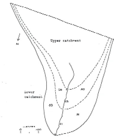
It is almost 30 years since I wrote my first distributed hydrological model for my PhD thesis, following the Freeze and Harlan (1969) blueprint but using finite element methods. My thesis (Beven, 1975) contained an application of the model to the small East Twin catchment in the UK, the catchment that had been studied in the field by Weyman (1970). The model represented a catchment as a number of variable width, slope following, hillslope segments, each represented by a 2D (vertical and downslope directions) solution of the Richards equation (Fig. 1). Computer limitations meant that only a coarse finite element mesh
could be used; even then, on the computers available, it proved difficult to perform simulations that took less computer time than real time simulated.
The modelling results were never published. They were simply not good enough. The model did not reproduce the stream discharges, it did not reproduce the measured water table levels, it did not reproduce the observed heterogeneity of inputs into the stream from the hillslopes (Fig. 2). It was far easier at the time to publish the results of hypothetical simulations (Beven, 1977). The ideas in what follows are essentially a distillation of those early experiences and of thinking hard about how to do distributed modelling in some sense “properly” since then.
discretisation of the flow domains has improved dramatically since 1975. However, just as in numerical weather forecasting, there remain limits to the detail that can be represented and there remains a problem of representing or parameterising sub-grid scale processes. As computer power improves further into the future, the feasible discretisation will become finer but the problem of sub-grid parameterisation does not go away. The form of that parameterisation might become simpler at finer scale but there is then the problem of knowing what might be the actual values of parameters for all the different spatial elements (Beven, 1989, 1996b, 2000a).
[image:2.595.75.266.66.297.2]There is then an interesting question as to how far such models, with their necessary approximations of processes and parameters at the element scale, can represent reality. An analysis of this question reveals a number of issues. These will be summarised here as the problems of nonlinearity; of scale; of uniqueness; of equifinality; and of uncertainty. The aim is, as ever, a “realistic” representation of the hydrology of a catchment that will be useful in making predictions in situations that have not yet occurred or where measurements have yet to be made. Indeed, one argument for the use of distributed modelling in hydrology has always been that they might be more “realistic” than simpler models that are calibrated to historical data in a curve-fitting exercise, with no guarantee, therefore, that they might do well in simulating responses in other periods or other
Fig. 1. The East Twin catchment, UK (21 ha), showing the hillslopes
segments for the finite element model of the Lower Catchment. Triangles show stream gauges.
conditions (e.g. Beven and O’Connell, 1982; Beven, 1985). That argument continues to be used in discussions of the problems of parameter estimation (e.g. Smith et al., 1994; De Marsily, 1994; Beven et al., 2001).
What then does “realism” mean in the context of distributed hydrological modelling? At the risk of making a gross generalisation, I suggest that most practising environmental scientists have, as a working philosophy, a pragmatic or heuristic realism; that the quantities that we deal with exist independently of our perceptions and empirical studies of them, that this extends even to quantities that are not (yet) observable, and that further work will move the science towards a more realistic description of the world. Again, at the risk of generalising, I would suggest that most practising environmental scientists do not worry too much about the theory-laden nature of their studies, (subsuming any such worries within the general framework of the critical rationalist stance that things will get better as studies progress). As has been pointed out many times, this theory laden-ness applies very much to experimental work, but it applies even more pointedly to modelling work where theory must condition model results very strongly.
This pragmatic realism is a “natural” philosophy in part because, as environmental scientists, we are often dealing with phenomena that are close to our day-to-day perceptions of the world. At a fundamental level I do a lot of computer modelling but I think of it as representing real water. If I try to predict pollutant transport, I think of it as trying to represent a real pollutant. Environmental chemists measure the characteristics of real solutions and so on. What I am calling pragmatic realism naturally combines elements of objectivism, actualism, empiricism, idealism, instrumentalism, Bayesianism, relativism and hermeneutics; of multiple working hypotheses, falsification, and critical rationalism (but allowing adjustment of auxiliary conditions); of confirmation and limits of validity; of methodologies of research programmes while maintaining an open mind to paradigm shifts; and of the use of “scientific method” within the context of the politics of grant awarding programmes and the sociology of the laboratory. Refined and represented in terms of ideals rather than practice, it probably comes closest to the transcendental realism of Bhaskar (1989; see also Collier, 1994). However, in hydrology at least, the practice often appears to have more in common with the entertaining relativism of Feyerabend (1991), not least because theories are applied to systems that are open which, as Cartwright (1999) has recently pointed out even makes the application of the equation
force=mass*acceleration difficult to verify or apply in
Fig. 2. Results of finite element simulations of the Lower East Twin catchment. All observed data collected by Darrell
Weyman. (a) Observed and predicted water table levels above a 1m wide throughflow trough. (b) Observed and predicted discharges from the throughflow trough using only measured soil parameter. (c) Observed and predicted discharges from the catchment. Dashed line: observed discharge from Upper catchment (not simulated). Dotted line: observed discharge from upper catchment with simulated discharge from lower catchment added. Full line: observed
discharge measured at outlet from lower catchment.
(a)
(b)
(c)
and energy balance equations in open systems (Beven, 2001b, d). This does not, of course, mean that such principles or laws should not be applied in practice, only that we should be careful about the limitations of their domain of validity (as indeed are engineers in the application of the force equation).
It is in the critical rationalist idea that the description of reality will continue to improve that many of the problems of environmental modelling have been buried for a long time. This apparent progress is clearly the case in many
The problem of nonlinearity
The problem of nonlinearity is at the heart of many of the problems faced in the application of distributed modelling concepts in hydrology, despite the fact that for many years “linear” models, such as the unit hydrograph and more recent linear transfer functions, have been shown to work well (see, for example, Beven 2001a), particularly in larger catchments (but see Goodrich et al., 1995, for a counter-example in a semi-arid environment where channel transmission losses result in greater apparent nonlinearity with increasing catchment size). In fact, this apparent linearity is often a
de facto artefact of the analysis. It applies only to the
relationship between some “effective” rainfall inputs and river discharge (and sometimes only to the “storm runoff” component of discharge). It does not apply to the relationship between rainfall inputs and river discharge that is known to be a nonlinear function of antecedent conditions, rainfall volume, and the (interacting) surface and subsurface processes of runoff generation. Hydrological systems are nonlinear and the implications of this nonlinearity should be taken into account in the formulation and application of distributed models.
This we do attempt to do, of course. All distributed models have nonlinear functional relationships included in their local element scale process descriptions of surface and subsurface runoff generation, whether they are based on the Richards equation or the SCS curve number. We have not been so good at taking account of some of the other implications of dealing with nonlinear dynamical systems, however. These include, critically, the fact that nonlinear equations do not average simply and that the extremes of any distribution of responses in a nonlinear system may be important in controlling the observed responses. Crudely interpreted in hydrological terms, this means local subgrid-scale nonlinear descriptions, such as Richards equation, should not be used at the model element scale (let alone at the GCM grid scale) where the heterogeneity of local parameter variations is expected to be important (Beven, 1989, 1995). The local heterogeneities will mean that the element scale averaged equations must be different from the local scale descriptions; that using mean local scale parameter values will not give the correct results, especially where there are coupled surface and subsurface flows (Binley
et al., 1989); and that the extremes of the local responses
(infiltration rates, preferential flows, areas of first saturation) will be important. This suggests, for example, that the use of pedotransfer functions to estimate a set of average soil parameters at the element scale of a distributed hydrological model should not be expected to give accurate results. Note: this follows purely from considerations of nonlinear
mathematics, even if Richards’ equation is acceptable as a description of the local flow processes (which could also be debated, e.g. Beven and Germann, 1982).
These implications are well known, so why have they been ignored for so long in distributed modelling in hydrology? Is it simply because there is no “physically based” theory to put in the place of Richards equation, since alternative sub-grid parameterisations seem too “conceptual” in nature? The recent work by Reggiani et al. (1998, 1999, 2000) is an attempt to formulate equations at the subcatchment or flow element scale directly in terms of mass, energy and momentum equations but has not solved the problem of parameterising the space and time integrated exchanges between elements in heterogeneous flow domains.
There are other implications of nonlinearity that are known to be important. Nonlinear systems are sensitive to their initial and boundary conditions. Unconstrained they will often exhibit chaotic behaviour. Initial and boundary conditions are poorly known in hydrology (see notably Stephenson and Freeze, 1974), as often are the observed values with which the model predictions are compared, but fortunately the responses are necessarily constrained by mass and energy balances. It is these constraints that have allowed hydrological modellers to avoid worrying too much about the potential for chaos. Essentially, by maintaining approximately correct mass and energy balances, models cannot go too far wrong, especially after a bit of calibration of parameter values. That does not mean, however, that it is easy to get very good predictions (even allowing for observation error), especially for extreme events.
This is reinforced by recent work in nonlinear dynamics looking at stochastically forced systems of simple equations. This work suggests that where there is even a slight error in the behaviour or attractor of an approximate model of a (known) system, the model will not be able to reproduce correctly the extremes of the distribution of the output variables either for short time scales or for integrated outputs over long (e.g. annual) time scales. If this is true for simple systems, does it imply that the same should be true for flood prediction and water yield predictions using (always slightly wrong) distributed models in hydrology? How can predictive capability be protected against these effects of nonlinearity?
The problem of scale
catchment area, even before trying to make some assessment of the nature and heterogeneity of the surface and subsurface processes with the measurement techniques available. It is clear, for example, that we have kept the Richards equation approach as a subgrid scale parameterisation for so long because it is consistent with the measurement scales of soil physical measurements. Because we have no measurement techniques that give information directly at the element grid scales (say 10 m to 1 km in the case of distributed hydrological models to 5 to 100 km in the case of land surface parameterisations for NWP and GCM models) we have not developed the equivalent, scale consistent, process descriptions that would then take account implicitly of the effects of subgrid scale heterogeneity and nonlinearity.
A recent comment by Blöschl (2001) has discussed the scale problem in hydrology. His analysis has much the same starting point as that of Beven (1995). He also recognises the need to identify the “dominant process controls” at different scales but comes to a totally different conclusion. Whereas Beven (1995) suggests that scaling theories will ultimately prove to be impossible and that is therefore necessary to recognise the scale dependence of model structures, Blöschl (2001) suggested that it is in resolving the scale problem that the real advances will be made in hydrological theorising and practice in the future. How do these two viewpoints bear on the application of distributed hydrological models?
Let us assume for the moment that it might be possible to develop a scaling theory that would allow the definition of grid or element scale equations and parameter values on the basis of knowledge of the parameter values at smaller scales. Certainly some first attempts have been made to do so in subsurface flows (e.g. Dagan, 1986, and others) and surface runoff (e.g. Tayfur and Kavvas, 1998). Attempts are also being made to describe element scale processes in terms of more fundamental characteristics of the flow domain, such as depositional scenarios for sedimentary aquifers. This reveals the difference between hydrology and some other subject areas in this respect. In hydrology, the development of a scaling theory is not just a matter of the dynamics and organisation of the flow of the fluid itself. In surface and subsurface hillslope hydrology, the flow is always responding to the local pore scale or surface boundary conditions. The characteristics of the flow domain determine the flow velocities. Those characteristics must be represented as parameter values at some scale. Those parameter values must be estimated in some way. But the characteristics are impossible to determine everywhere, even for surface runoff if it occurs. For subsurface flow processes the characteristics are essentially unknowable with current measurement techniques. Thus, they must be inferred in some way from
either indirect or large scale measurements. In both cases, a theory of inference would be required. This would be the scaling theory but it is clear from this argument that any such theory would need to be supported by strong assumptions about the nature of the characteristics of the flow domain even if we felt secure about the nonlinearities of the flow process descriptions. The assumptions would not, however, be verifiable: it is more likely that they would be made for mathematical tractability rather than physical realism and applied without being validated for a particular flow domain because, again, of the limitations of current measurement techniques.
Thus, the problem of scale in distributed hydrological modelling does not arise because we do not know the principles involved. We do, if we think about it, understand a lot about the issues raised by nonlinearities of the processes, heterogeneities of the flow domains, limitations of measurement techniques, and the problem of knowing parameter values or structures everywhere. The principles are general and we have at least a qualitative understanding of their implications, but the difficulty comes in the fact that we are required to apply hydrological models in particular catchments, all with their own unique characteristics.
The problem of uniqueness
In the last 30 years of distributed hydrological modelling there has been an implicit underlying theme of developing a general theory of hydrological processes. It has been driven by the pragmatic realist philosophy outlined earlier. The idea that if we can get the description of the dynamics of the processes correct then parameter identification problems will become more tractable is still strongly held. However, in a recent paper, I have put forward an alternative view: that we should take much more account of the particular characteristics of particular catchment areas, i.e. to consider the question of uniqueness of place much more explicitly (Beven, 2000a).
measurement errors. However, such a model must still have some way of taking account of all the local heterogeneities of the flow domain in any application to a particular catchment. In short, even the perfect model has parameters that have to be estimated.
Presumably, the perfect model will embody within it some expressions to relate the parameter values it requires to some measureable characteristics of the flow domain (indeed, the perfect model seems to require that a scaling theory is, in fact, feasible). This could be done in either a disaggregation or aggregation framework. A disaggregation framework would require making inferences from catchment scale measurements to smaller scale process parameters. This would be similar to the type of calibration exercise against catchment discharges that is often carried out today. It clearly leaves scope for multiple parameter sets being able to reproduce the catchment scale behaviour in a way that is consistent with the model dynamics.
An aggregation process implies that information will be required on the heterogeneity of parameter values within the catchment area. We will not, however, be able to determine those parameters everywhere in a particular catchment area with its own unique characteristics, especially because the perfect model would tell us that it is the extremes of the distribution of characteristics that may be important in controlling storm runoff generation. It is always more difficult to estimate the extremes of a distribution than the first two moments (even where the distribution can be characterised in simple form). Thus, a very large number of measurements would be required without any real guarantee that they are spatially coherent. Since our current measurement techniques have severe limitations in assessing spatial variability then it would seem that the aggregation approach would also result in a large number of model parameter sets being consistent with the model dynamics in reproducing the large scale behaviour.
Thus, even if we knew the structure of the perfect model, uniqueness of place leads to a very important identifiability problem. In the case of the perfect model, this could be considered as simply a problem of non-identifiability i.e. a unique (“optimal”) set of parameters would exist, if only we had the measurements available to be able to identify it. In practice, with limited measurements available there would most probably be a non-uniqueness problem i.e. that there appear to be several or many different optimal parameter sets but the measurements do not allow us to distinguish between them. However, we cannot normally assume that we are using such a perfect model structure. Thus, Beven (1993, 1996a,b) has suggested that it is better to approach the problem of uniqueness of place using a concept of
equifinality of model structures and parameter sets. This
choice of word is intended to indicate an explicit recognition that, given the limited measurements available in any application of a distributed hydrological model, it will not be possible to identify an “optimal” model. Rather, we should accept that there may be many different model structures and parameter sets that will be acceptable in simulating the available data.
It is worth stressing in this that, even if we believed that we knew the perfect model structure, it would not be immune to the problem of equifinality in applications to particular catchments with their own unique characteristics. Limited measurements, and particularly the unknowability of the subsurface, will result in equifinality, even for the perfect model.
There has been a commonly expressed hope that, in the future, remote sensing information would lead to the possibility of more robust estimates of spatially distributed parameter values for distributed hydrological modelling in applications to unique catchment areas. Pixel sizes for remote sensing are at the same scale, or even sometimes finer, than distributed model element scales and in many images we can easily detect visually spatial patterns that appear to be hydrologically significant (we can include here ground probing radar and cross-borehole tomography techniques that give some insight into the local nature of the subsurface flow domain). However, the potential for remote sensing to provide the information required would appear to be limited. The digital numbers stored by the sensor do not give direct estimates of the hydrogical variables or parameters required at the pixel scale. They require an interpretative model. Such a model will, itself, require parameter values to reflect the nature of the surface, the structure and state of the vegetation, the state of the atmosphere, etc. In fact, the digital numbers received by the user may already have been processed by an interpretative model to correct for atmospheric effects etc. in a way that may not reflect all the processes involved even if the interpretative model is physically “realistic”. The user may wish to leave such corrections to the imaging “experts”, but will then need to apply a further interpretative model for the hydrological purposes he/she has in mind. The resulting uncertainties may, at least sometimes, be very significant (see for example Franks et al., 1997), especially where the parameters of the interpretative model might also be expect to change over time, e.g. with vegetation growth or senescence.
emissions, to models of the subsurface. However, it is worth repeating that it is often possible to see hydrologically significant patterns in some images. Thus, it should be expected that there is useful information on the distributed responses of particular hillslopes and catchments to be gained from remote sensing, but it will certainly not solve the problem of uniqueness.
The problem of equifinality
The recognition of equifinality arose out of Monte Carlo experiments in applying models with different parameter sets in simulating catchment scale discharges (Beven and Binley, 1992; Duan et al., 1992; Beven, 1993). It resulted in some interestingly different responses. The University of Arizona group response was that a better method for identifying the optimal parameter set was required, leading to their development of the stochastic complex evolution methodology, as embodied in the UA-SCE software. Other experiments in global optimisation have explored simulated annealing, genetic algorithms and Monte Carlo Markov Chain methodologies (e.g. Kuczera, 1997, Kuczera and Parent, 1999). A further recognition that the results of even a global optimisation depended strongly on the evaluation measure used has lead to the exploration of multi-objective optimisation techniques such as the Pareto optimal set methodology of Yapo et al. (1998) and Gupta et al. (1999), again from the Arizona group. The underlying aim, however, has still been to identify parameter sets that are in some sense optimal.
The response of the Lancaster University group was different. They were prepared to reject the idea that an optimal model would ever be identifiable and develop the concept of equifinality in a more direct way. This lead to the Generalised Likelihood Uncertainty Estimation (GLUE) Methodology (Beven and Binley, 1992; Beven et al., 2000, Beven, 2001a). GLUE is an extension of the Generalised Sensitivity Analysis of Hornberger, Spear and Young (Hornberger and Spear, 1981; Spear et al., 1994) in which many different model parameter sets are chosen randomly, simulations run, and evaluation measures used to reject some models (model structure/parameter set combinations) as
non-behavioural while all those considered as non-behavioural are
retained in prediction. In GLUE the predictions of the behavioural models are weighted by a likelihood measure based on past performance to form a cumulative weighted distribution of any predicted variable of interest. Traditional statistical likelihood measures can be used in this framework, in which case the output prediction distributions can be considered as probabilities of prediction of the variable of interest. However, the methodology is general in that more
general likelihood measures, including fuzzy measures, can be used in which case only conditional prediction limits or possibilities are estimated. Different likelihood measures can be combined using Bayes equation or a number of other methods (Beven et al., 2000; Beven, 2001a).
There is one other implication of equifinality that is of particular importance in distributed modelling. Distributed models have the potential to use different parameter values for every different element in the spatial discretisation. In general this means that many hundreds or thousands of parameter values must be specified. Clearly it is not possible to optimise all these parameter values, they must be estimated on the basis of some other information, such as soil texture, vegetation type, surface cover etc. Values are available for different types of soil, vegetation etc in the literature. However, such values will themselves have been back-calculated or optimised against observations gathered in specific (unique) locations under particular sets of forcing conditions. One of the lessons from GLUE studies is that it is the parameter set that is important in giving a good fit to the observations. It is very rarely the case that the simulations are so sensitive to a particular parameter that only certain values of that parameter will give good simulations. More often a particular parameter value will give either good or bad simulations depending on the other parameter values in the set. Thus, bringing together different parameter values from different sources is no guarantee that, even if they were optimal in the situations where they were determined, they will give good results as a set in a new set of circumstances. Be warned!
The problem of uncertainty
The aim of the GLUE methodology is to produce a set of behavioural models that properly reflect the uncertainties arising from the modelling process and that reproduce the observed behaviour of the catchment within the limitations of measurement error. This is not always easy because of errors in the input data and errors in the model structure, both of which may be difficult to assess a priori. This is demonstrated quite nicely in the simulation results of Freer
et al. (1996) where a timing error in the initiation of
snowmelt in the model results in a long period where the GLUE model prediction limits parallel but do not bracket the observations. This could of course be corrected, either by adding a stochastic error model or, if the interest is in short term forecasting, by data assimilation.
and the problem of defining a model for that type of uncertainty. Thus, again, the results will be conditional: conditional on the input sequences used, the model structures considered, the random parameter sets chosen, and the likelihood measures chosen for model evaluation. All these choices, however, must be made explicit and can be subject to critical review by end-users (and reviewers).
In simulation, the use of a stochastic error model raises some interesting issues. It should be expected that the structure of the modelling errors should vary over time. This has long been recognised in terms of the heteroscedasticity of errors but, in hydrological series, it should also be expected that the errors will be non-gaussian and changing in skew between high and low flows. Thus it may be difficult to formulate a statistical error model (and likelihood function) that is consistent over both time and, with the GLUE methodology, for different behavioural parameter sets that may also vary locally in their bias and error covariance structures. So much of statistical parameter inference is predicated on the implicit assumption that the “true” model is available, that the rejection of that possibility in favour of a concept of equifinality means that some new approaches are needed. GLUE is one such approach that can be used for models for which it is computationally feasible. It has been used for distributed and semi-distributed models over limited domains but clearly there are still some distributed modelling problems for which the parameter dimensionality and computational times mean that a full Monte Carlo analysis remains infeasible. However, it is an open question as to whether the affordable parallel computer power to do so will arrive before we develop the conceptual and theoretical developments or measurement techniques that might make a GLUE-type analysis unnecessary.
One response to the equifinality problem is to suggest that the problem only arises because we are using poor models (Beven, 1996a). Again, there is a widespread belief that if we could get the model dynamics right then perhaps we would have less parameter identification problems. The analysis above suggests that this belief is not justified. Even the perfect model will be subject to the problem of equifinality in applications and we know very well that we have not quite attained the perfect model. Clearly, therefore, we are using poor models in that sense but many modern modellers, as instrumentalists, will argue that despite their limitations they are the best models available (often giving quite acceptable simulations) and they are what we must make use of in practical prediction. Thus, it is perhaps best to view the uncertainty arising from equifinality as a question of decidability. The fact that we have many models that give acceptable simulations of the available data does not mean that they are poor models. It only means that they cannot be
rejected (are not decidable) on the basis of the data to hand. Additional data, or different types of data, might mean that we could reject more of the models that up to now have been behavioural in this sense.
In some cases new data might mean that we could reject all the models we have available, in which case we might have to revise the model structures or potential parameter sets considered in the analysis. In this case we could actually gain understanding. If models continue to work acceptably well but cannot be distinguished then there is really no way of deciding between them. If we have to reject models then we will gain much more information about what might be an appropriate process description. If we have to reject all models then we will have to query the model structure itself, or look more closely at how meaningful are the observations that we are using to decide on model rejection. However, rejection of all models will also mean that we have no predictions, so we might (just possibly) instead choose to relax our criteria for retaining models as “acceptable”.
Is there a way ahead? How far can we go?
Looking at the problem of equifinality as a question of decidability allows an interesting reformulation of the GLUE approach, to the extent that Beven (2001b) has suggested that it allows an Alternative Blueprint for distributed model in hydrology, to replace that of Freeze and Harlan (1969). It is not, however, an alternative set of descriptive equations. The discussion above suggests that, although we know that the Freeze and Harlan description is inadequate, we do not yet have the measurement techniques that would enable us to formulate a new scale dependent set of process descriptions. Thus we will have to resort to the variety of conceptual formulations that are currently available (this includes Richards equation which, as applied as a sub-grid parameterisation in practice, is certainly a conceptual model that should be expected to have scale dependent parameter values, Beven, 1989, 1996b).end-users of hydrological predictions would take a similar view.
However, my own view is that there is actually an opportunity here to put hydrological prediction on a firmer scientific basis (see Beven, 2000a). Let us pursue the idea of equifinality as a problem of decidability given the available data a little further. The idea of accepting many behavioural models in prediction because they have all given simulations that are consistent with the available data does not mean that those models are indistinguishable, nor that we could not decide between those models given the right sort of data. This is perhaps best viewed in terms of a mapping of the landscape of a catchment into the model space (Beven, 2000a, b, 2001b). Accepting the concept of equifinality, each landscape unit might be represented by many different behavioural models in the model space. The mapping will therefore be an uncertain or fuzzy mapping depending on what type of evaluation measures are used, with different landscape units mapping into possibly overlapping areas of the model space. The differences in predicted behaviour for the behavioural models for each landscape unit can then be reflected in mapping the results of simulations in the model space.
One of the interesting features of this view of the modelling processes is that, in principle, everything is known about the simulations in the model space. If the models are run purely deterministically with a single set of input forcing data this will be a one to one mapping. But even if the model is stochastic and the inputs are treated stochastically then the output statistics could still be mapped in the model space, subject only to computational constraints. Thus differences in predicted behaviour in the model space can be identified and an exploration of the model space might then provide the basis for setting up some testable hypotheses that might allow some of the behavioural models to be rejected on the basis of a new data collection programme within an underlying falsificationist framework. The approach is then analogous to that of multiple working hypotheses (the behavioural models) with an experimental programme designed to differentiate between them and (hopefully) falsify or reject some of them. This might then be represented as hydrological science to the end-user and/or research grant awarding agency.
It is this process that forms the Alternative Blueprint of Beven (2001b). The Alternative Blueprint as method can be summarised by the following six stages:
(i) Define the range of model structures to be considered. (ii) Reject any model structures that cannot be justified as physically feasible a priori for the catchment of interest.
(iii) Define the range for each parameter in each model. (iv) Reject any parameter combinations that cannot be
justified as physically feasible a priori.
(v) Compare the predictions of each potential model with the available observed data (which may include both catchment discharge and internal state measurements, as well as any qualitative information about catchment processes) and reject any models which produce unacceptable predictions, taking account of estimated error in the observations.
(vi) Make the desired predictions with the remaining successful models to estimate the risk of possible outcomes.
In terms of the assessment of physically realistic distributed models in hydrology the most important steps in this process are the rejection of models that cannot be considered as physically feasible, either a priori, or as resulting in unrealistic predictions.
There is an interesting further stage that might prove to be useful in the future. If, in principle, a model structure or set of model structures has an adequate range of hydrological functionality and that functionality can be mapped in the model space for a certain set of input conditions then the areas of different functional response can be mapped out in the model space. Thus, it may only be necessary to make representative predictions for these different functionally similar areas of the feasible model space and not for all possible models in the feasible space, thereby increasing the computational efficiency of the methodology, at least in prediction. The definition of what constitutes functional similarity is, of course, an issue and will undoubtedly vary with the aims of a project. A first attempt at the application of such a strategy, in the context of defining land surface to atmosphere fluxes over a heterogeneous landscape, has been outlined by Franks et al. (1997; see also Beven and Franks, 1999).
Some unresolved questions……
new conceptual developments are unlikely to happen quickly but can incorporate them easily as necessary. Indeed, it may be that conceptual model developments are most likely to happen when we are forced to reject all the available models because of inconsistency with data.
There remain many unresolved questions that must be addressed in distributed modelling in the future. A collection of such questions arose out of the Francqui Workshop on the future of distributed modelling in hydrology held in Leuven in April 2000 (see Beven, 2000b, Beven and Feyen, 2001). Some of the most important, relevant here, include: how far do we need to consider the detail in processes descriptions when there is no way to measure the local detail necessary to support such descriptions? Can a model, for example, based on a hysteretic storage discharge relationship for a hillslope be just as physically acceptable as the local hysteresis in soil moisture characteristics required by a full local application of the Richards equation (or, in the structure of the Alternative Blueprint would you reject it a priori as physically infeasible)?
A further question arises in applications requiring distributed predictions (for example of the extent of flood inundation, of the risk of erosion, of potential source areas for non-point pollution, etc). If it is accepted that accuracy in local predictions must be necessarily limited, when would predictions of where rather than how much be acceptable. In some cases, such as those noted above, a relative assessment of the spatial distribution of risk, including an assessment of uncertainty, might be sufficient for risk based decision making.
There are still relatively few assessments of distributed models that have included spatially distributed observations in either calibration or evaluation. Most assessments are still based on comparisons of observed and predicted discharges alone. This is perfectly understandable given the time and effort required in gathering the spatial data sets necessary but it is really not acceptable (for a fine example of a study that has made assessments of spatial predictions see Uhlenbrook and Leibundgut, 2001). As Klemeš (1986) pointed out, even split record tests of models based on discharge data alone are not a strong test of model feasibility for lumped models, let alone distributed models. However, the intention to test the spatial predictions of a distributed model raises further questions. What sort of data should be collected as a useful and cost effective test? How best to make use of spatial data that might already be available, for example from observation wells or soil moisture profiles, when there may be a mismatch in scales between the observations and the predicted variables? What sort of evaluation or likelihood measures should be used when the errors may be variable in structure in space and time? Can
the spatial data be used to suggest different model structures where predictions of current model structures are shown to be deficient? These questions can be posed within the Alternative Blueprint but will require commitment in applications of the methodology to detailed data sets.
Finally, there is a real question as to how to develop distributed models that properly reflect the collective intelligence of the hydrological community. At first sight it would appear that one major store of collective intelligence is in the model software systems of the current generation of distributed models. I would venture to suggest, however, that the continued application of models based on the Freeze and Harlan blueprint is not an indication of much collective intelligence (Beven, 2001e). It is a simple response to the fact that no coherent alternative has been proposed over the last 30 years. “Progress” in that time has consisted in trying available distributed models to see if they work with more or less calibration and little reporting of cases where they have failed in their spatial predictions (though the graphics have certainly improved). It remains to be seen if new model structures will develop out of new measurements (remote sensing, tomographic imaging, incremental stream discharges etc.) becoming available, but in the short term this seems unlikely. Where then is the collective intelligence of the hydrological community stored? There appear to be two more important depositories. One is the back issues of journals relevant to hydrology, including journals in complementary fields (soil science, plant physiology, nonlinear dynamics, etc); the other the field data sets that have been collected from experimental and operational catchments over the years. It does seem at the current time that not much is being made of either of these sources of information and that a fundamental review of what is necessary information for the development of future distributed models is needed.
It is, perhaps, opportune at this point to return to my PhD thesis and the East Twin catchment. In his 1970 paper on the results of field studies in the East Twin, Darrell Weyman noted:
“To produce a control section discharge of 12 litres/sec by throughflow alone from 540 m of bank requires a mean peak throughflow discharge of 1320 cm3/min/metre. In contrast the peak discharge from the soil [throughflow] plots was only 185 cm3/min/metre. On the other hand, measured seeps from the soil at other locations on the channel gave peak discharges for this storm of up to 7800 cm3/min. The supply area for these inputs is indeterminate but in terms of bank length is certainly not more than one metre as seep spacing is often less than that distance.” (p.31)
the Alternative Blueprint, would the existing models all be rejected a priori at this site? Think about it in respect of both principle and practice (and the naivety of a young graduate student)!
……and a vision for the future
The Alternative Blueprint, outlined briefly above and in Beven (2001b), provides a framework for doing distributed modelling as hydrological science in a consistent way and in the face of the various adversities faced by the modeller. It is useful, within the sociology of science, to have such a methodology as a defence against criticism of the apparently
ad hoc nature of some of the models that are reported,
especially those that use conceptual model elements to interpret the information available from GIS overlays. However, distributed models are not only being developed because the computational resources, object oriented programming languages, graphical interfaces, and spatial databases of today make it a relatively easy task to implement such models, but because there is a demand for practical prediction of the effects of land use change, of non-point source pollution, of the risks and impacts of erosion, and so on. The future of distributed modelling lies, in fact, not so much in the development of new theories for scaling or process representation but in the application of models and their use over a period of time in specific catchments.
This is very important because long term use in specific catchments implies an increasing potential for model evaluation, post-simulation audits, and learning about where the model does not work. This suggests that including an assessment of predictive uncertainty in modelling studies will be a good idea for the modeller since it allows a greater possibility of being “right”, or at least of being wrong gracefully. It also suggests that, over time, there should be a greater possibility of learning about the uniqueness of different places within an application area, building up that knowledge, both qualitative and quantitative, in a form that can be used to refine the representation of functional responses within the framework of the Alternative Blueprint. This will be one way of making use of the increased computer power that will be available in the future: to build a system that will store or re-run the results of past simulations in a form that can be compared with a current situation; to identify where there is drift or error in the simulations or where the model functionality seems inadequate; to act as a repository for information, knowledge and understanding about specific catchment areas such that local model representations of those areas can be improved.
This does not imply that such a system, focussed on the details of specific catchments, should not take new
developments in modelling into account. Clearly, if some radical change in modelling concepts is achieved in the future, perhaps driven by new measurement techniques, then there should be the potential to include it. The challenge will be to make a system that is “future proof” in this respect, not only with respect to such new developments but also to the change of people who will run it and to changes in the computer systems on which it might run. Then, gradually, we will gain more real understanding about how local hydrological systems really work, including all their local complexities. It is now possible to model the hydrology of the globe (albeit with some uncertainty). More modestly and more importantly it should also now be possible to model places on that globe in detail: still with uncertainty, but gradually learning about their particular characteristics and particular idiosyncracies in hydrological response.
Acknowledgements
This paper is an extended version of the Dalton Medal lecture given at the EGS XXVI General Assembly at Nice in March 2001. One does not get to give such a lecture without being in debt to a great number of people and I would particularly like to thank Mike Kirkby who sent me in the right direction as an undergraduate and post-doc; Jim McCulloch who gave me a job at the Institute of Hydrology as a mathematical modeller in spite of my degree in geography; George Hornberger for all the discussions about modelling while I was teaching at the University of Virginia; and Peter Young who invited me to Lancaster and has kept my attention on the data as a source of information, even if he does not approve of my use of the word likelihood. Then there are the many collaborators and friends who have contributed ideas and support, especially Tom Dunne, Eric Wood, Andrew Binley, Bruno Ambroise, Charles Obled, Sarka Blazkova, André Musy and Jan Feyen, as well as the several generations of Lancaster graduate students and post-docs who have actually done the real work, of whom Jim Freer has suffered the longest. Thanks are also due to the Francqui Foundation for their support for the International Chair held at K.U. Leuven in 1999/2000 and to NERC for supporting work on distributed modelling and the GLUE methodology.
References
Beven, K.J., 1975. A deterministic spatially distributed model of
catchment hydrology, PhD thesis, University of East Anglia,
Norwich.
Beven, K.J., 1977. Hillslope hydrographs by the finite element method. Earth Surf. Process, 2, 13-28.
Beven, K.J., 1989. Changing ideas in hydrology: the case of physically based models. J. Hydrol., 105, 157-172.
Beven, K.J., 1993, Prophecy, reality and uncertainty in distributed hydrological modelling, Adv. Water Resour., 16, 41-51 Beven, K.J., 1995. Linking parameters across scales: sub-grid
parameterisations and scale dependent hydrological models,
Hydrol. Process, 9, 507-526.
Beven, K.J., 1996a. Equifinality and Uncertainty in Geomorphological Modelling, In: The Scientific Nature of
Geomorphology, B.L. Rhoads and C.E. Thorn (Eds.), Wiley,
Chichester, UK. 289-313.
Beven, K.J., 1996b. A discussion of distributed modelling, Chapter 13A, In: Distributed Hydrological Modelling, J-C. Refsgaard and M.B. Abbott (Eds.) Kluwer, Dordrecht, 255-278. Beven, K.J., 2000a. Uniqueness of place and the representation of
hydrological processes, Hydrol. Earth System Sci., 4, 203-213. Beven, K.J., 2000b. On the future of distributed modelling in
hydrology, Hydrol.Process. (HPToday), 14, 3183-3184. Beven, K.J., 2001a. Rainfall-Runoff Modelling – the Primer, Wiley,
Chichester, UK. 356pp.
Beven, K.J., 2001b. Towards an alternative blueprint for a physically-based digitally simulated hydrologic response modelling system, Hydrol. Process., 15, in press
Beven, K.J., 2001c. On landscape space to model space mapping,
Hydrol. Process. (HPToday), 15, 323-324.
Beven, K.J., 2001d. On hypothesis testing in hydrology,
Hydrological Processes (HPToday), in press.
Beven, K.J., 2001e. On modelling as collective intelligence,
Hydrological Processes (HPToday), in press
Beven, K.J. and Germann, P., 1982. Macropores and water flow in soils, Water Resour. Res., 18, 1311-1325.
Beven, K.J. and O’Connell, P.E., 1982. On the role of physically-based distributed models in hydrology. Institute of Hydrology
Report, No. 81, Wallingford, UK.
Beven, K.J. and Binley, A.M., 1992. The future of distributed models: model calibration and uncertainty prediction, Hydrol.
Proces., 6, 279-298.
Beven, K.J. and Franks, S.W., 1999. Functional similarity in landscape scale SVAT modelling, Hydrol. Earth System Sci., 3, 85-94.
Beven, K.J., Freer, J., Hankin, B. and Schulz, K., 2000. The use of generalised likelihood measures for uncertainty estimation in high order models of environmental systems. In: Nonlinear
and Nonstationary Signal Processing, W.J. Fitzgerald, R.L.
Smith, A.T. Walden and P.C. Young (Eds.). CUP, Cambridge, UK. 115-151.
Beven, K.J., Musy, A. and Higy, C., 2001. Tribune Libre: L’unicité de lieu, d’action et de temps, Revue des Sciences de l’Eau, in press.
Beven, K.J. and Feyen, J., 2001. Preface to Special Issue on The Future of Distributed Modelling, Hydrol. Process., 15, in press. Binley, A.M., Beven, K.J. and Elgy, J., 1989. A physically-based model of heterogeneous hillslopes. II. Effective hydraulic conductivities. Water Resour. Res., 25, 1227-1233.
Bhaskar, R., 1989. Reclaiming Reality, Verso, London
Blöschl, G., 2001, Scaling in hydrology, Hydrol. Process.
(HPToday), 15, 709-711.
Cartwright, N., 1999. The Dappled World: a Study of the
Boundaries of Science, Cambridge University Press, Cambridge.
247pp
Collier, A., 1994. Critical Realism, Verso, London. 276pp Dagan, G., 1986. Statistical theory of groundwater flow and
transport: pore to laboratory; laboratory to formation and formation to regional scale, Wat. Resour. Res., 22, 120-135. De Marsily, G., 1994, Quelques réflexions sur l’utilisation des
modèles en hydrologie, Revue des Sciences de l’Eau, 7, 219-234.
Duan, Q.S., Sorooshian, S. and Gupta, V., 1992. Effective and efficient global optimisation for conceptual rainfall-runoff models, Water Resour. Res., 28, 1015-1031.
Feyerabend, P., 1991. Three dialogues on knowledge, Blackwell, Oxford, UK.
Franks, S. and Beven, K.J., 1997. Estimation of evapotranspiration at the landscape scale: a fuzzy disaggregation approach, Water
Resour. Res., 33, 2929-2938.
Freer, J., Beven, K.J. and Ambroise, B., 1996. Bayesian estimation of uncertainty in runoff prediction and the value of data: an application of the GLUE approach, Water Resour. Res., 32, 2161-2173.
Freeze, R.A. and Harlan, R.L., 1969. Blueprint for a physically-based, digitally-simulated hydrologic response model, J. Hydrol.,
9, 237-258.
Goodrich, D.C., Lane, L.J., Shillito, R.M., Miller, S.N., Syed, K.H. and Woolhiser, D.A., 1997. Linearity of basin response as a function of scale in a semiarid watershed, Water Resour. Res.,
33, 2951-2965.
Gupta, H.V., Sorooshian, S. and Yapo, P.O., 1999. Towards improved calibration of hydrologic models: multiple and noncommensurable measures of information, Water Resour.Res.,
34, 751-763.
Hornberger, G.M. and Spear, R.C., 1981. An approach to the preliminary analysis of environmental systems, J. Environ.
Manage., 12, 7-18.
Klemeš, V., 1986. Operational testing of hydrologic simulation models, Hydrol. Sci. J., 31, 13-24.
Kuczera, G., 1997. Efficient subspace probabilisitc parameter optimisation for catchment models, Water Resour. Res., 33, 177-186. Kuczera, G. and Parent, E., 1998. Monte Carlo assessment of parameter uncertainty in conceptual catchment models: the Metropolis algorithm, J. Hydrol., 211, 69-85.
Reggiani, P., Sivapalan, M. and Hassanizadeh, S.M., 1998. A unifying framework for watershed thermodynamics: balance equations for mass, momentum, energy and entropy and the second law of thermodynamics, Adv. Water Resour., 23, 15-40. Reggiani, P., Hassanizadeh, S.M., Sivapalan, M. and Gray, W.G., 1999. A unifying framework for watershed thermodynamics: constitutive relationships, Adv. Water Resour., 23, 15-40. Reggiani, P., Sivapalan, M. and Hassanizadeh, S.M., 2000.
Conservation equations governing hillslope responses: exploring the physical basis of water balance, Water Resour. Res., 36, 1845-1863.
Smith, R.E., Goodrich, D.R., Woolhiser, D.A. and Simanton, J.R., 1994. Comments on “Physically-based hydrologic modelling. 2. Is the concept realistic?” by R.B. Grayson, I.D. Moore and T.A. McMahon, Water Resour. Res., 30, 851-854.
Spear, R.C., Grieb, T.M. and Shang, N., 1994. Parameter uncertainty and interaction in complex environmental models,
Water Resour. Res., 30, 3159-3170.
Stephenson, R. and Freeze, R.A., 1974. Mathematical Simulation of Subsurface Flow Contributions to Snowmelt Runoff, Reynolds Creek, Idaho, Water Resour Res, 10, 284-298.
Tayfur, G. and Kavvas, M.L., 1998, Areally-averaged overland flow equations at hillslope scale, Hydrol. Sci. J., 43, 361-378. Uhlenbrook, S. and Leibundgut, Ch., 2001. Process-oriented catchment modelling and multiple response validation, Hydrol.
Process., 15, in press.
Yapo, P.O., Gupta, H.V. and Sorooshian, S., 1998. Multi-objective global optimisation for hydrologic models, J. Hydrol., 204, 83-97.