On the uncertainty of stream networks derived from elevation data: the error propagation approach

www.hydrol-earth-syst-sci.net/14/1153/2010/ doi:10.5194/hess-14-1153-2010

© Author(s) 2010. CC Attribution 3.0 License.

Earth System

Sciences

On the uncertainty of stream networks derived from elevation data:

the error propagation approach

T. Hengl1, G. B. M. Heuvelink2, and E. E. van Loon1

1_{Institute for Biodiversity and Ecosystem Dynamics, University of Amsterdam, Nieuwe Achtergracht 166,}

1018 WV Amsterdam, The Netherlands

2_{Wageningen University and Research, P.O. Box 47, 6700 AA Wageningen, The Netherlands}

Received: 22 December 2009 – Published in Hydrol. Earth Syst. Sci. Discuss.: 29 January 2010 Revised: 18 June 2010 – Accepted: 18 June 2010 – Published: 2 July 2010

Abstract. DEM error propagation methodology is extended to the derivation of vector-based objects (stream networks) using geostatistical simulations. First, point sampled ele-vations are used to fit a variogram model. Next 100 DEM realizations are generated using conditional sequential Gaus-sian simulation; the stream network map is extracted for each of these realizations, and the collection of stream networks is analyzed to quantify the error propagation. At each grid cell, the probability of the occurrence of a stream and the propagated error are estimated. The method is illustrated us-ing two small data sets: Baranja hill (30 m grid cell size; 16 512 pixels; 6367 sampled elevations), and Zlatibor (30 m grid cell size; 15 000 pixels; 2051 sampled elevations). All computations are run in the open source software for statis-tical computingR: package geoRis used to fit variogram; package gstat is used to run sequential Gaussian simula-tion; streams are extracted using the open source GISSAGA via theRSAGAlibrary. The resulting stream error map (In-formation entropy of a Bernoulli trial) clearly depicts areas where the extracted stream network is least precise – usually areas of low local relief and slightly convex (0–10 difference from the mean value). In both cases, significant parts of the study area (17.3% for Baranja Hill; 6.2% for Zlatibor) show high error (H >0.5) of locating streams. By correlating the propagated uncertainty of the derived stream network with various land surface parameters sampling of height measure-ments can be optimized so that delineated streams satisfy the required accuracy level. Such error propagation tool should

Correspondence to: T. Hengl ([email protected])

become a standard functionality in any modern GIS. Re-maining issue to be tackled is the computational burden of geostatistical simulations: this framework is at the moment limited to small data sets with several hundreds of points. Scripts and data sets used in this article are available on-line via the www.geomorphometry.org website and can be easily adopted/adjusted to any similar case study.

1 Introduction

In geomorphometry, Digital Elevation Models (DEM) are routinely used to extract various continuous (gridded) land surface parameters, and/or discrete (vector) land surface ob-jects. Assuming that DEMs are perfectly accurate, extraction of land surface parameters and objects is a simple one itera-tion operaitera-tion (Fig. 1a). However, in reality, DEMs are not perfect representations of reality – DEMs suffer from sys-tematic and random errors and DEM elevations differ from what we measure on the field. In fact, errors are inevitable, even if elevation models are produced using highly accurate and dense sampling techniques such as LiDAR (Evans and Hudak, 2007; Bater and Coops, 2009). Errors are inherent both in measurements of elevations, and in the DEM analy-sis algorithms, and can possibly have a significant influence on the reliability of final products. By ignoring errors in the input layers, analysts often get disappointed when their prod-ucts are evaluated versus ground truth data. This is true espe-cially for hydrological applications (Wise, 2000; Wechsler, 2007).

Derive mean and

standard deviation Simulate

gridded DEM

Extract stream network

(a)

Filter spurious

sinks Generate

gridded DEM

Extract stream network

(b)

Estimate variogram

model Save

stream network for each realisation repeat m times

se

mivar

iance

distance

Filter spurious

sinks

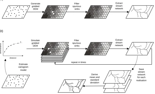
Fig. 1. Workflow scheme for stream extraction from elevation data: (a) assuming that elevations carry no uncertainty; (b) the Monte Carlo

error propagation approach withmrealizations. In this case, filtering of spurious sinks is specific to the case studies and not a general operation.

a way to assess the propagated uncertainty associated with the output of the analysis, is known as “error propagation” (Heuvelink, 1998). The potential of using error propaga-tion has been first recognized by Burrough (1986) and En-glund (1993). At that time, it seemed unlikely that stochastic simulations would become routinely available in a GIS en-vironment. Since then, the world has evolved: computers are more powerful, statistical tools are more accessible and more sophisticated. We are slowly reaching a point when er-ror propagation will become a standard toolbox of any GIS software (Wechsler, 2007). Examples of using error propa-gation methods to assess the accuracy of various scalar-type land surface parameters derived from DEMs can be found in the work of Fisher (1992); Heuvelink (1998); Dutta and Herath (2001); Raaflaub and Collins (2006) and Oksanen and Sarjakoski (2005). Brown and Heuvelink (2007) recently produced a generic library for uncertainty modeling called “Data Uncertainty Engine” (DUE). A group at Aston Univer-sity has been developing the Uncertainty Markup Language (UncertML, http://www.uncertml.org) that could become a standard for writing metadata for error propagation applica-tions. However, there are still technical and conceptual issues

2 Methods and materials

2.1 Error propagation

GIS error propagation can be defined as a set of statistical procedures that model uncertainties in the input maps, and for a given GIS operation, estimate the (propagated) error of mapping a feature of interest. In mathematical terms, the output map is a result of an operation applied to multiple spatial layers (Heuvelink, 1998):

U (s)=gA1(s),...,Ap(s) (1)

whereA1(s),...,Ap(s)are the GIS inputs (spatial layers),

U (s)is the output map,pis the number of inputs,s is the vector of coordinates (spatial locationx,y), andgis the GIS operation. The main focus of error propagation is determi-nation of the mean value (U (¯ s)) and its standard deviation (σ_U2(s)), or ideally the entire probability distribution of the output map U for any location s in the area of interest _A. Note that the probability distribution of the output map is quite involved because it must also capture the spatial sta-tistical dependencies. In case of GIS output that is a spa-tial object such as a streamline, the probability distribution is even more complex. Possibly the easiest way to charac-terize uncertainty of discrete spatial objects is by generating a number of those objects (especially for objects that cannot easily be specified): for example, river network is the output from numerical algorithm that operates on the terrain data; although the flow modeling formulas are deterministic, the consequent uncertainty can not be specified separately from the terrain on which it was generated. In fact, Tarboton and Baker (2009) argue that it is close to impossible to integrate uncertainty in the flow-algebra.

The benefit of running an error propagation analysis is, first and foremost, that it quantifies the uncertainty in the GIS result. If the probability distribution of the inputAis narrow, then we might expect that the propagated uncertainty will be narrow as well, but this need not always be the case. The sen-sitivity of model output to small changes in the input is also important. Also, when there are multiple uncertain inputs it becomes difficult to predict the impact of error in input maps on derived products. The situation is even more difficult if errors in inputs are spatially variable – in some parts of the study area they can be high, in others low – so that it becomes difficult to predict where in the study area the uncertainty of the derived map becomes critical. By ignoring the fact that errors in input maps exist and that they are significant, we create a wrong idea about the precision of the derived land surface objects. Hence the primary benefit of running error propagation is visual and statistical assessment of errors in the output maps.

In principle, there are two main approaches to error prop-agation: (a) the analytical, and (b) the Monte Carlo approach (Heuvelink, 2002). In the first case, the propagated error is derived using some mathematical technique such as via

a Taylor series expansion; in the second case, stochastic sim-ulation is used to samplemtimes from the input probabil-ity distribution and the operation is repeatedmtimes. The Monte Carlo approach is more suited for cases where the GIS operationgis so complex that it is practically impossible to mathematically derive the propagated distribution model. Since this is the case for many GIS applications, the Monte Carlo approach has become the dominant approach to error propagation (Wechsler, 2007; Poggio and Soille, 2008).

In the case of Monte Carlo simulation, the mean value (U (¯ s)) and the standard deviation (σ_U2(s)) of the output fea-ture is simply:

¯ U (s)=

Pm

j=1UjSIM(s)

m (2)

σU(s)=

v u u t

Pm

j=1

U_jSIM(s)− ¯U (s) 2

m−1 (3)

In the case of stream network extraction from DEMs, the error propagation model (Eq. 1) is:

USIM=gnzSIM,b1,...,bp

o

(4) wherezSIM is the simulated elevation map,USIM(s)is the output value of stream (either 1 or 0, depending on whether the location is part of the stream or not), andb1,...,bp are

the user-defined, constant, hydrological model parameters, for example: minimum segment length, initiation grid, initi-ation threshold etc. These parameters can be uncertain too. Although this looks like a trivial model, the functiong in-volves a spatial analysis with respect to flow direction on the input elevation map, so that small differences in elevation at some locations can result in completely different stream pat-terns while large differences at other locations can have no effect.

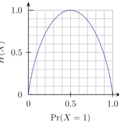
Streams have several specific properties that distinguish them for other land surface parameters and objects. Streams are discrete objects – a stream is composed of a set of in-terconnected points (represented as grid cells). These ob-jects have attributes such as length and curviness, Horton or Strahler ordering. A grid cell can be part of a stream (value 1) or not (value 0) i.e. it becomes a Bernoulli variable with probabilitypbeing part of the stream. The majority of cells will have a small value for p simply because streams are by definition rare events. The mean of the Bernoulli vari-able at some location is simplyp; its variance is given by p·(1−p). The uncertainty of detecting streams can be alter-natively characterized by the Shannon entropy (Shannon and Weaver, 1949):

Fig. 2. The uncertainty of deriving stream can be best described

using the information entropy (H) of a Bernoulli trial. This plot is courtesy of Brona Brejova, Comenius University in Bratislava, Slovakia.

stream at the cell, divided by the total number of Monte Carlo realizations. The precision of estimating the propagated un-certainty is inversely related to the Monte Carlo sample size. This means that if we run 100 simulations, and then at some location detect stream 99/100 times (p=0.99), the estimated error will be 0.056, and we can not map uncertainty with a finer precision. If the model detects streams with equal prob-ability of stream and not-stream (p=0.5), this will produce the highest error of 1 (Fig. 2).

2.2 Geostatistical simulations

Monte Carlo analysis of spatial error propagation requires the generation of realistic simulations of elevation values. The most common technique in geostatistics used to generate equiprobable realizations of a spatial feature is the Sequential Gaussian Simulation (Goovaerts, 1997). To simplify matters, it is assumed that elevation can be modeled as a stationary random function (Goovaerts, 1997; Kyriakidis et al., 1999) with a constant mean:

µ=_E{Z(s)} (6)

and a variogram model that only depends on distance be-tween points:

2·γ (h)=Var{Z(s)−Z(s+h)}

=_En[Z(s)−Z(s+h)]2o (7) wherehis the separation vector between two locations, and γ (h) is the semivariance. A capital letter Z is used be-cause we assume that the model is probabilistic, i.e. there is a range of equiprobable realizations of the same model. If the variable of interest (elevation) has been sampled at a set of point locations (z(s1),z(s2),. . . ,z(sn), wheresi=(xi,yi)),

then these can be used to fit a variogram model. Once we have estimated the variogram model parameters, we can use

this model to produce simulations ofZ that have the same spatial structure:

zSIM(s0)=E{Z(si)|z(si),i=1,...,n} (8)

where zSIM is the simulated value at location s0. In this

case, simulations will be conditioned on the observations at sampling locationsz(si). Under the assumption of

second-order stationarity, we can use for example a global exponen-tial variogram with three parameters to produce a simulated DEM. A slightly more sophisticated variogram is the Mat´ern variogram model, which has an additional parameter to de-scribe the smoothness (Stein, 1999; Minasny and McBrat-ney, 2005):

γ (h)=C0·δ (h)+C1·

₁

2v−1_·0(v)·

_h R

v ·Kv·

_h R

(9) whereC0, is the nugget parameter,C1the sill parameter,R

the range parameter,δ (h)is the Kronecker delta,Kvis the

modified Bessel function,0is the gamma function andvis the smoothness parameter. The Mat´ern variogram model is especially suited for elevation data because the smoothness, common for topographic features, can be nicely represented with thev-parameter. Note, however, that using the Mat´ern variogram is only sensible when the nugget variance is in-significant i.e. close to zero.

When additional auxiliary maps are available that can be used to explain the deterministic component in the spatial distribution of elevation values, more accurate simulations of topography can be produced using the regression-kriging model (Hengl et al., 2008). For the purpose of this article, we will follow a simple case and assume: (a) that the elevation values are realizations of a second-order stationary random function with a constant trend; and (b) that the spatial auto-correlation can be modeled using a Mat´ern variogram.

In summary, the error propagation approach to extraction of streams from elevation data can be summarized in five steps (Fig. 1b):

1. calculate an experimental variogram from the data and fit a Mat´ern variogram model (with parameters:C0,C1,

Randv) to represent the variability of the input DEM; 2. generate multiple realizations of the DEM using

condi-tional simulation and the variogram model fitted previ-ously (Eq. 8);

3. filter spurious sinks; derive stream network for each re-alization, and save the temporary result (Eq. 4); 4. aggregate the derived maps to estimate stream

occur-rence frequency and error of mapping streams (Eq. 5); 5. evaluate how the propagated error relates to various

A disadvantage of the Monte Carlo approach is that it re-quires a significantly large number of realizations to produce a reliable estimate of the distribution function. The num-ber of realizationsmmust be sufficiently large to obtain sta-ble results, but exactly how largemshould be depends on how accurate the results of the uncertainty analysis should be. Theoretically speaking, the accuracy of the Monte-Carlo method is proportional to the square root of the number of runsm(Temme et al., 2008). Therefore, to double the ac-curacy one must quadruple the number of runs. This means that although many runs may be needed to reach stable and accurate results, any degree of precision can be reached by taking a large enough samplem. As a rule of thumb, we can take 100 simulations as being large enough, and everything below 20 as insufficient (Heuvelink, 1998). Consequently, the Monte-Carlo method is computationally demanding, par-ticularly when the GIS operation takes much computing time (Heuvelink, 2002).

2.3 Software tools

In this article we use a combination of statistical and geo-graphical computing software to assess propagated error of detecting streams: SAGAGIS for geographical computing, and R for statistical computing; all operations are in fact combined in the same script. In this case,Ris used to control both internal add-on packages, but also external GISSAGA (R“on top”) via a special link libraryRSAGA. A detailed description ofR+SAGAintegration can be can be found in Brenning (2008).

Because most of the packages used in this article are not common to majority of GIS users and hydrologists (espe-cially to users of ESRI-products), we consider worth intro-ducingSAGA,gstatandgeoR, and reviewing its main func-tionality. A small guide on how to install, set and make first steps in the two packages, is also given in the Appendix A. This should help you reproduce the analysis shown in this ar-ticle with your own data. Even more detailed instructions on how to combineRandSAGAusing the same data sets can be found in Hengl (2009).

2.3.1 SAGAGIS

SAGA1 (System for Automated Geoscientific Analyses) is an open source GIS that has been developed since 2001 at the University of G¨ottingen (the group recently collectively moved to the Institut f¨ur Geographie, University of Ham-burg), Germany, with the aim to simplify the implementation of new algorithms for spatial data analysis (Conrad, 2006, 2007). A point data set of measured elevations can be used inSAGAto generate a Digital Elevation Model (DEM), that can then be used to extract a stream network (see scheme in Fig. 1a). For example, you can open the point layer inSAGA

1_{http://saga-gis.org}

GIS, then use the module Grid7→Gridding7→Spline inter-polation7→Thin Plate Splines (local) and generate a smooth DEM. Then, you can preprocess the DEM to remove spuri-ous sinks using the method of Planchon and Darboux (2001). Select Terrain Analysis7→Preprocessing7→Fill sinks, and then set the minimum slope parameter to 0.1.

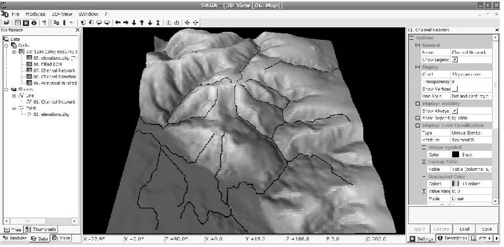
Once you have prepared a DEM, you can derive stream networks using the Channel Network function which is avail-able inSAGAunder Terrain Analysis7→Channels. This im-plements the original algorithm described in Conrad (2007) and which is based on the FD8 multiple flow direction algo-rithm by Quinn et al. (1995). As a result, you should get a map shown in Fig. 3. Assuming that the DEM and the stream extraction model are absolutely accurate, i.e. that they per-fectly fit the reality, this would then be the end product of the analysis (which corresponds to the scheme in Fig. 1a). 2.3.2 Rand packagesgstatandgeoR

Ris the command-based environment for statistical comput-ing (R Development Core Team, 2009). Many spatial pack-ages have been contributed in the past 3–4 years, which allow Rto be also used for spatial analysis. Two important add-on packages that are used in this article aregstat(Pebesma, 2004) andgeoR(Diggle and Ribeiro Jr., 2007). In principle, a large part of functionality ofgstatandgeoRoverlap. On the other hand,geoRhas many original methods, including an original format for spatial data (calledgeodata). geoR is especially powerful to fit variograms (including interactive visual fitting), and for dealing with non-normal data; gstat is somewhat more fit to run predictions and generate simula-tions, even with large data sets.gstatalso uses spatial classes inR, so that conversion to GIS formats is fairly easy.

Once we have simulated mDEMs using gstat, we can derive stream networks using the “Channel Network” func-tion, which is available also via the command line – via the

ta channelsSAGAlibrary (see further Appendix A). This means that, through scripting inR, one can automate both geographical processing and statistical analysis, and imple-ment the computational scheme shown in Fig. 1b to any sim-ilar data set.

2.4 Study areas and data sets

Fig. 3. Stream network generated inSAGAGIS using standard settings. In this case we used 40 (pixels) as the minimum length of streams. Case study Baranja Hill; viewed from the West side.

The study area “Baranja hill” is located in eastern Croa-tia (centered at 45◦₄₈0_16.441200_{N, and 18}◦₃₉0_54.19800_{E); it}

has been extensively mapped over years and several GIS lay-ers are available at various scales (Hengl and Reuter, 2008). The study area corresponds approximately to the size of a single 1:20 000 aerial photo. Its main geomorphic features include hill summits and shoulders, eroded slopes of small valleys, valley bottoms, a large abandoned river channel, and river terraces (Fig. 3). Elevation of the area ranges from 80 to 240 m with an average of 157.6 m and a standard deviation of 44.3 m. The data set consists of 6367 points of field mea-sured heights. The complete data set is available for down-load from the geomorphometry dataset repository2. A simi-lar error propagation exercise using the same case study can be followed in Temme et al. (2008).

The second case study, “Zlatibor”, is located in the South-western part of Serbia (centered at 43◦43044.600N and 19◦42037.800E). The area is mainly hilly plateau, with the ex-ception of the north-eastern part where the slopes are much steeper (see further Fig. 6b). Elevations range from 850 m to a maximum of 1174 m; the total size of the area is 13.5 square kilometers. The data set consists of 2051 height measure-ments. An additional set of 1020 very precise spot heights used for error assessment is also available. This data set is described in detail in Hengl et al. (2008) and can be also ob-tained from the geomorphometry dataset repository3.

2_{http://geomorphometry.org/content/baranja-hill} 3_{http://geomorphometry.org/content/zlatibor}

3 Results

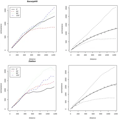
The first result of analysis are the variogram models fitted ingeoR(Fig. 4). These show that the target variable (z) in general varies equally in all directions in both study areas. This is especially distinct for shorter distances (<500 m), which allows us to model the variograms using isotropic models. For Baranja Hill study areageoRfits a Mat´ern var-iogram model with nugget parameter C0=0, sill parameter

C1=1831, and range parameter R=1051 m (practical range

is 3.1 km); for Zlatibor case study, the elevation values are more variable – nugget parameter is stillC0=0, the sill

pa-rameter isC1=2173, range parameter isR=761 m. In both

caseszseems to be a relatively smooth variable – there is no nugget variation and spatial autocorrelation is effective (practical range) up to distance of 2–3 km.

Both are in fact typical variograms for elevation data i.e. representation of a land surface. Note also that, in both cases, the target variable shows close to normal distribution so no transformation was necessary. As expected, the confidence bands (envelopes) are much narrower at smaller distances (Fig. 4). The relatively wide confidence bands at larger dis-tances indicate that it might be worthwhile to consider using local (moving window) geostatistical analysis and adjust the variogram parameters locally.

0 200 400 600 800 1000 1200

0

500

1000

1500

distance

semiv

ar

iance

0° 45° 90° 135°

BaranjaHill

● ●

● ●

● ● ●

● ●

● ●

● ●

0 200 400 600 800 1000 1200

0

500

1000

1500

2000

2500

distance

semiv

ar

iance

0 200 400 600 800 1000 1200

0

500

1000

1500

2000

distance

semiv

ar

iance

0° 45° 90° 135°

Zlatibor

● ●

● ●

● ●

● ●

● ● ●

● ●

0 200 400 600 800 1000 1200

0

500

1000

1500

2000

2500

distance

semiv

ar

iance

Fig. 4. Variograms fitted for Baranja hill (above) and Zlatibor case studies (below); left: anisotropy in four directions; right: isotropic Mat´ern

variogram model fitted using the weighted least squares (WLS) and its confidence bands.

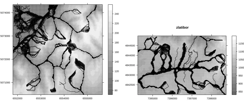
other. The 100 realizations of stream network maps for the two study areas are shown in Fig. 5. The visualization of density of streams clearly illustrates the concept of propa-gated uncertainty. If you zoom in into this map, you will notice several things. First, in some areas streams are iso-lated and hence seem to be very improbable; in other areas stream are densely distributed but over a wider area. Note also that the derived streams follow the gridded-structure of the DEMs, which explains some artificial breaks in the lines. Some artifacts in these maps are probably a consequence of the fact that we have used arbitrary input parameters for the minimum length of streams (40) and initial grid. These pa-rameters could have been find-tuned by experts familiar with the study areas, but this is not relevant for this exercise.

BaranjaHill

5071000 5072000 5073000 5074000

6552000 6553000 6554000 6555000

80 100 120 140 160 180 200 220 240

zlatibor

4842500 4843000 4843500 4844000 4844500

7395000 7396000 7397000 7398000

850 900 950 1000 1050 1100 1150

Fig. 5. 100 realizations of stream network overlaid on top of each other: left: Baranja hill case study; right: Zlatibor case study. The greyscale

legends indicates elevations in meters.

N

N

(a) (b)

0.00 0.25 0.50 0.75 1.00

Fig. 6. Propagated error of mapping streams estimated using Eq. (5); visualized inSAGAGIS: (a) Baranja hill case study; (b) Zlatibor case study. The lines indicate the true streams – digitized from topo maps.

stream. The results from these two small case studies clearly demonstrates the usefulness of the error propagation analysis – by mapping the propagated error we can delineate the most problematic areas and focus our further efforts.

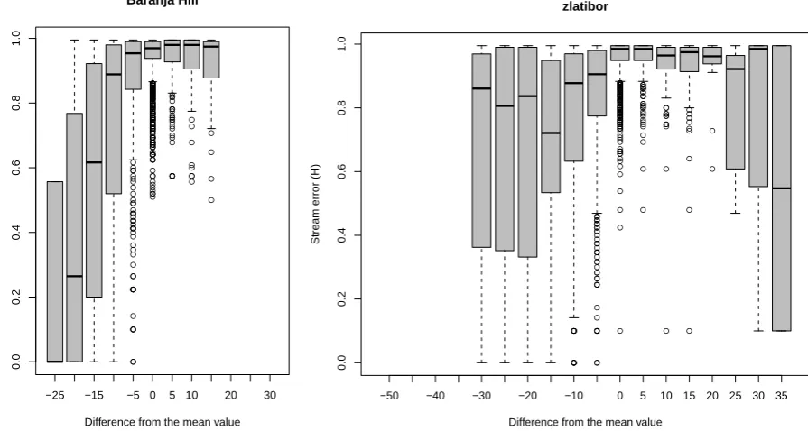
Now that we have estimated the propagated uncertainty of extracting channel networks (streams) from DEMs, we can try to understand how this uncertainty relates to the ge-omorphology of terrain. It is interesting to derive a map of channel-slope and/or topographic wetness index, as it largely controls the hydrological properties, and the difference from the mean value in 5×5 search radius, as it describes local variability of shapes.

● ● ● ● ● ● ● ● ● ● ● ● ● ● ● ● ● ● ● ● ● ● ● ● ● ● ● ● ● ● ● ● ● ● ● ● ● ● ● ● ● ● ● ● ● ● ● ● ● ● ● ● ● ● ● ● ● ● ● ● ● ● ● ● ● ● ● ● ● ● ● ● ● ● ● ● ● ● ● ● ● ● ● ● ● ● ● ● ● ● ● ● ● ● ● ● ● ● ● ● ● ● ● ● ● ● ● ● ● ● ● ● ● ● ● ● ● ● ● ● ● ● ● ● ● ● ● ● ● ● ● ● ● ● ● ● ● ● ● ● ● ● ● ● ● ● ● ● ● ● ● ● ● ● ● ● ● ● ● ● ● ● ● ● ● ● ● ● ● ● ● ● ● ● ● ● ● ● ● ● ● ● ● ● ● ● ● ● ● ● ● ● ● ● ● ● ● ● ● ● ● ● ● ● ● ● ● ● ● ● ● ● ● ● ● ● ● ● ● ● ● ● ● ● ● ● ● ● ● ● ● ● ● ● ● ● ● ● ● ● ● ● ● ● ● ● ● ● ● ● ● ● ● ● ● ● ● ● ● ● ● ● ● ● ● ● ● ● ● ● ● ● ● ● ● ● ● ● ● ● ● ● ● ● ● ● ● ●

−25 −15 −5 0 5 10 20 30

0.0 0.2 0.4 0.6 0.8 1.0 Baranja Hill

Difference from the mean value

Stream error (H)

● ● ● ● ● ● ● ● ● ● ● ● ● ● ● ● ● ● ● ● ● ● ● ● ● ● ● ● ● ● ● ● ● ● ● ● ● ● ● ● ● ● ● ● ● ● ● ● ● ● ● ● ● ● ● ● ● ● ● ● ● ● ● ● ● ● ● ● ● ● ● ● ● ● ● ● ● ● ● ● ● ● ● ● ● ● ● ● ● ● ● ● ● ● ● ● ● ● ● ● ● ● ● ● ● ● ● ● ● ● ● ● ● ● ● ● ● ● ● ● ● ● ● ● ● ● ● ● ● ● ● ● ● ● ● ● ● ● ● ● ● ● ● ● ● ● ● ● ● ● ● ● ● ● ● ● ● ● ● ● ● ● ● ● ● ● ● ● ● ● ● ● ● ● ● ● ● ● ● ● ● ● ● ● ● ● ● ● ● ● ● ● ● ● ● ● ● ● ● ● ● ● ● ● ● ● ● ● ● ● ● ● ● ● ● ● ● ● ● ● ● ● ● ● ● ● ● ● ● ● ● ● ● ● ● ● ● ● ● ● ● ●

−50 −40 −30 −20 −10 0 5 10 15 20 25 30 35

0.0 0.2 0.4 0.6 0.8 1.0 zlatibor

Difference from the mean value

Stream error (H)

Fig. 7. Bar plots showing relationship between the relative relief (difference from the mean value in the 5×5 search radius) and cumulative errors. In both cases the highest errors of mapping streams are in slightly convex areas (positive values in range 0–10).

of locating streams in the area of relatively high relief (Zlat-ibor), however, the spatial accuracy of derived streams does not get better than±50 m, so that it is reasonable to consider degrading the scale of the output map e.g. from 1:15 000 to 1:50 000 scale.

The computational burden of this method is also an issue. The most costly operations are geostatistical simulations and extraction of stream networks. Geostatistical simulations, even with a search radius of only 30 closest points, takes 5–10 min to generate 100 simulations for these small study areas (150×100 pixels). This means that this framework is at the moment limited to small data sets with few hundreds of points; it would be probably of limited use for large LiDAR point data sets.

4 Discussion and conclusions

The two case studies demonstrate that it is worth investing in error propagation – in both cases we are able to detect some difficult areas where extracted stream networks will be criti-cally imprecise. Figures 5 and 6 show two interesting things: (1) the dispersion of stream networks is in some areas signif-icant; (2) streams are especially difficult to map in low-relief areas where the difference from the mean value is positive – meaning areas with convex shapes. This largely reflects our expectation, but it is rewarding to be able to prove these as-sumptions using hard data. Our results correspond with the results of Poggio and Soille (2008) who discovered that

un-certainty of stream segments is in general significant and es-pecially high for Strahler order one or two. Some remaining issues and ideas for further research are discussed below.

We have also limited the number of simulations to 100. Perhaps this number should be larger, particularly because we are dealing with a feature that commonly has a smallp. It should be feasible to evaluate the increase in accuracy with an increasing number m, e.g. by evaluating the change in derived probability or attribute property such as estimated stream length or catchment width. If such a parameter or function does not change anymore below a certain threshold, no more simulations seem to be required. An elegant alterna-tive can be to calculate the information content of each addi-tional realization. With an increasing sample size, the change in the ultimate probability field becomes less and less. This is certainly an idea worth further research.

We have also set the grid cell size at 30 m without any real justification. The next step would be to consider some statistically sound approach to select a grid cell size based on the accuracy of the derived stream network. This follows the idea of Hutchinson (1996), who use an iterative DEM cell-size optimization algorithm as implemented in the ANU-DEM package. By plotting the error of mapping streams versus the grid spacing index, one can select the grid cell size that shows the maximum information content in the fi-nal map. The optimal grid cell size is the one where further refinement does not change the accuracy of derived streams. It would be interesting to see if the optimal detection of the grid cell size for hydrological objects can be operationalized, so that the users only need to provide the point data.

Another question that needs to be addressed is how much of the analysis should be automated? Can and should error propagation be automated so that it becomes a default opera-tion of any DEM analysis? If yes, users will not even have to see the steps behind error propagation (black-box approach), but simply select a land surface object/parameter of interest and the software will decide about the reasonable number of simulations, suitable grid cell size, depict the areas that are critical etc. The case studies shown in this paper are fairly small in size, hence it was not expensive to run 100 simulations. How to deal with the computational complexity of error propagation? These case studies obviously demon-strated that such analysis provides richer picture of the spatial variability of propagated errors, but is this always needed? What if error propagation is useful only for small parts of the study area; is there then still a need to run such analysis globally? How would geostatistical simulation + error propa-gation techniques perform with LiDAR surveys that consists of millions of points? Are results of error propagation very dependent on the type of data (field survey, LiDAR, SRTM DEM etc.) or will the spatial patterns of uncertainty be dif-ferent?

The two case studies shown in this article consists of pre-cisely measured elevations over a small and homogenous area with relatively constant variogram parameters. How to generate simulated DEMs when a spatial auto-correlation structure model (variogram) is not available or differs lo-cally? Traditionally, geostatistical techniques are developed

to work with point-sampled values. For DEMs generated di-rectly from a scanning device (e.g. SRTM DEM) it is a se-rious problem to get a reliable estimate of a variogram. In addition, uncertainty of measured elevations is heavily de-pendent on the type of land use (local spatial auto-correlation structure), hence simulated DEMs should reflect this prop-erty also. A solution to generate simulations of e.g. SRTM DEM is the co-kriging framework. Separate estimation of the variogram and cross-variogram parameters for the error surface and the main signal in the DEM is rather inexpensive, but simulations using co-kriging are even more computation-ally intensive.

There is also an issue of how to represent the outputs of error propagation. Should the land surface object derived us-ing error propagation represented as fuzzy objects? Should we abandon concept of absolutely discrete land surface ob-jects at first place? If yes, which data structure should be used to save and exchange such objects? Or is the spaghetti rep-resentation shown in Fig. 5 more informative? Tøssebro and Nyg˚ard (2008) provide a probabilistic framework for com-puting uncertainties for simple geographic objects such as points and unstructured lines, but how could these be com-bined with geostatistical simulations?

Floor for discussion is open and everybody is welcome to contribute. For the beginning, software developers can try implementing error propagation frameworks as standard toolboxes to extract information from elevation data. The users can further consider testing this framework in areas of variable relief, surface roughness and with elevation mea-surements from various sources. We anticipate that the mean challenge of the proposed framework will be processing of the LiDAR data that is typically very large and requires lo-calization of analysis. With the further advances of technol-ogy (computing power) and geostatistics (local variograms), both operations should become feasible.

Appendix A

Installation and first steps withR+SAGA

The following text provides instructions how to obtain and installSAGAandRand implement the analysis described in this article with your own data. R+SAGAcan be run on Windows™ and Linux operating systems. Mac OS™ version ofSAGAis still under development.

Start with installingRand its spatial packages. Visit the Rproject homepage4and obtain the recent installation from CRAN. After you finish installingR, open the new session and install the contributed packages: select the Packages7→ Install package(s) from the main menu. Note that, if you wish to install a package on the fly, you will need to select a suitable CRAN mirror from where it will download and un-pack a un-package. Another quick way to get all un-packages used

inRto do spatial analysis5 (as explained in Bivand et al., 2008) is to install thectvpackage and then execute the com-mand:

> install.packages("ctv") > library(ctv)

> install.views("Spatial")

This will allow most of the spatial packages available forR, includingmaptools,rgdal,gstat,geoR, andRSAGA.

Next, if you are a Windows™ user, obtain theSAGA bi-naries from a Source Forge repository. SAGAGIS is a full-fledged GIS with support for raster and vector data. It in-cludes a large set of geoscientific algorithms (over 300 mod-ules), being especially powerful for the analysis of DEMs. With the release of version 2.0 in 2005, SAGAworks un-der both Windows and Linux operating systems. In addition, SAGAis an open-source package, which makes it especially attractive to users that would like extend or improve its exist-ing functionality. To installSAGAsimply unzip the binaries to your program files directory. Then openSAGAGUI and test its functionality using point-and-click operations. Now you can consider switching to the scripting environment. Go to yourRsession and load theRSAGAlibrary:

> library(RSAGA)

First check ifRis able to locateSAGAon your machine: > rsaga.env()

$workspace [1] "."

$cmd

[1] "saga_cmd.exe"

$path

[1] "C:/Progra˜1/saga_vc"

$modules

[1] "C:/Progra˜1/saga_vc/modules"

which means that you can now send operations fromR to SAGA. Open themodulesfolder under theSAGAdirectory and you will notice a large number of DLL libraries. To get an info what can a certain module do, type:

> rsaga.get.modules("ta_channels")

$ta_channels

code name interactive

1 0 Channel Network FALSE

2 1 Watershed Basins FALSE

3 2 Watershed Basins (extended) FALSE

4 3 Vertical Distance to CN FALSE

5 4 Overland Flow Distance to CN FALSE

6 5 D8 Flow Analysis FALSE

7 6 Strahler Order FALSE

8 NA <NA> FALSE

9 NA <NA> FALSE

5_{http://cran.r-project.org/web/views/Spatial.html}

Next, we need to get the list of parameters needed to extract channel network from a DEM map:

> rsaga.get.usage("ta_channels", 0)

SAGA CMD 2.0.4

library path: C:/Progra˜1/saga_vc/modules library name: ta_channels

module name : Channel Network

Usage: 0 -ELEVATION <str> [-SINKROUTE <str>] -CHNLNTWRK <str> -CHNLROUTE <str>

-SHAPES <str> -INIT_GRID <str>

[-INIT_METHOD <num>] [-INIT_VALUE <str>] [-DIV_GRID <str>] [-DIV_CELLS <num>] [-TRACE_WEIGHT <str>] [-MINLEN <num>]

-ELEVATION:<str> Elevation Grid (input)

-SINKROUTE:<str> Flow Direction Grid (optional input)

-CHNLNTWRK:<str> Channel Network Grid (output)

-CHNLROUTE:<str> Channel Direction Grid (output)

-SHAPES:<str> Channel Network Shapes (output)

-INIT_GRID:<str> Initiation Grid Grid (input)

-INIT_METHOD:<num> Initiation Type Choice

Available Choices: [0] Less than [1] Equals [2] Greater than

-INIT_VALUE:<str> Initiation Threshold Floating point

-DIV_GRID:<str> Divergence Grid (optional input)

-DIV_CELLS:<num> Tracing: Max. Divergence Integer

Minimum: 1.000000

-TRACE_WEIGHT:<str> Tracing: Weight Grid (optional input)

-MINLEN:<num> Min. Segment Length

Finally, you can generate a stream network shown in Fig. 3 using thersaga.geoprocessor:

> rsaga.geoprocessor(lib="ta_channels", + module=0, param=list(ELEVATION="DEM.sgrd", + CHNLNTWRK="tmp.sgrd",

+ CHNLROUTE="tmp.sgrd", + SHAPES="streams.shp", + INIT_GRID="DEM.sgrd", + DIV_CELLS=3, MINLEN=40))

SAGA CMD 2.0.4

library path: C:/Progra˜1/saga_vc/modules library name: ta_channels

Load grid: DEM.sgrd... ready

Load grid: DEM.sgrd... ready

Parameters

Grid system: 30; 128x 129y; 6551817x 5070464y Elevation: DEM.sgrd Flow Direction: [not set]

Channel Network: Channel Network Channel Direction: Channel Direction Channel Network: Channel Network Initiation Grid: DEM.sgrd

Initiation Type: Greater than Initiation Threshold: 0.000000 Divergence: [not set]

Tracing: Max. Divergence: 3 Tracing: Weight: [not set] Min. Segment Length: 40

Channel Network: Pass 1 Channel Network: Pass 2 Channel Network: Pass 3 Create index: DEM.sgrd ready

Channel Network: Pass 4 Channel Network: Pass 5 Channel Network: Pass 6 ready

ready

Save grid: tmp.sgrd... ready

Save grid: tmp.sgrd... ready

Save shapes: streams.shp... ready

Save table: streams.dbf... ready

More detail on how to produce results shown can be found in theRscript, available via www.geomorphometry.org.

Acknowledgements. This article evolved from a two-day workshop

entitled “Automated analysis of elevation data in R” that was held at the University of Z¨urich on 29 and 30 August 2009. The prin-cipal author of this article would like to thank the Geomorphome-try conference organizers Ross Purves and Stephan Gruber (Depart-ment of Geography) for hosting this workshop, and Carlos Grohm-man for kindly helping us run this workshop. The authors would also like to thank all the workshop participants for their com-ments and suggestions. Join the open source initiative by sending your ideas/suggestion via theR-sig-geomailing list and/or via the geomorphometry-organized meetings.

Edited by: P. Molnar

References

Bater, C. and Coops, N.: Evaluating error associated with lidar-derived DEM interpolation, Comput. Geosci., 35, 289–300, 2009.

Bivand, R., Pebesma, E., and Rubio, V.: Applied Spatial Data Anal-ysis with R, Use R Series, Springer, Heidelberg, 14–15, 2008. Brenning, A.: Statistical Geocomputing combining R and SAGA:

The Example of Landslide susceptibility Analysis with gen-eralized additive Models, in: SAGA – Seconds Out, edited by: B¨ohner, J., Blaschke, T., and Montanarella, L., vol. 19, Hamburger Beitr¨age zur Physischen Geographie und Land-schafts¨okologie, 23–32, 2008.

Brown, J. and Heuvelink, G.: The Data Uncertainty Engine (DUE): a software tool for assessing and simulating uncertain environ-mental variables, Comput. Geosci., 33, 172–190, 2007. Burrough, P.: Principles of Geographical Information Systems for

Land Resources Assessment, Oxford University Press, Oxford, 241–264, 1986.

Conrad, O.: SAGA – Program Structure and Current State of Im-plementation, in: SAGA – Analysis and Modelling Applications, edited by: B¨ohner, J., McCloy, K. R., and Strobl, J., vol. 115, Verlag Erich Goltze GmbH, 39–52, 2006.

Conrad, O.: SAGA – Entwurf, Funktionsumfang und Anwendung eines Systems f¨ur Automatisierte Geowissenschaftliche Analy-sen, PhD thesis, University of G¨ottingen, G¨ottingen, 2007. Diggle, P. J. and Ribeiro Jr., P. J.: Model-based Geostatistics,

Springer Series in Statistics, Springer, 51–53, 2007.

Dutta, D. and Herath, S.: Effect of DEM Accuracy in Flood Inunda-tion SimulaInunda-tion using Distributed Hydrological Models, Seisan Kenkyu, 53, 602–605, 2001.

Englund, E.: Spatial Simulation: Environmental Applications, in: Environmental modeling with GIS, edited by: Goodchild, M., Parks, B., and Steyaert, L., chap. 43, Oxford University Press, New York, 432–446, 1993.

Evans, J. S. and Hudak, A. T.: A multiscale curvature filter for iden-tifying ground returns from discrete return lidar in forested envi-ronments, IEEE T. Geosci. Remote., 45, 1029–1038, 2007. Fisher, P.: First experiments in viewshed uncertainty:

Simulat-ing fuzzy viewsheds, Photogramm. Eng. Rem. S., 58, 345–352, 1992.

Goovaerts, P.: Geostatistics for Natural Resources Evaluation (Ap-plied Geostatistics), Oxford University Press, New York, 380– 392, 1997.

Hengl, T.: A Practical Guide to Geostatistical Mapping, University of Amsterdam, Amsterdam, 221–239, 2009.

Hengl, T. and Reuter, H.: Geomorphometry: Concepts, Software, Applications, vol. 33 of Developments in Soil Science, Elsevier, Amsterdam, 26–29, 2008.

Hengl, T., Bajat, B., Reuter, H., and Blagojevi´c, D.: Geostatistical modelling of topography using auxiliary maps, Comput. Geosci., 34, 1886–1899, 2008.

Heuvelink, G. B. M.: Error Propagation in Environmental Mod-elling with GIS, Taylor & Francis, London, UK, 35–46, 1998. Hutchinson, M. F.: A locally adaptive approach to the interpolation

of digital elevation models, in: Proceedings of the Third Inter-national Conference/Workshop on Integrating GIS and Environ-mental Modeling, National Center for Geographic Information and Analysis, Santa Barbara, CA, p. 6, 1996.

Kyriakidis, P. C., Shortridge, A. M., and Goodchild, M. F.: Geo-statistics for Conflation and Accuracy Assessment of Digital El-evation Models, Int. J. Geogr. Inf. Sci., 13, 677–708, 1999. Minasny, B. and McBratney, A. B.: The Mat´ern function as a

gen-eral model for soil variograms, Geoderma, 128, 192–207, 2005. Oksanen, J. and Sarjakoski, T.: Error propagation of DEM-based

surface derivatives, Comput. Geosci., 31, 1015–1027, 2005. Pebesma, E. J.: Multivariable geostatistics in S: the gstat package,

Comput. Geosci., 30, 683–691, 2004.

Planchon, O. and Darboux, F.: A fast, simple and versatile algo-rithm to fill the depressions of digital elevation models, Catena, 46, 159–176, 2001.

Poggio, L. and Soille, P.: Quality assessment of hydro-geomorphological features derived from Digital Terrain Models, EUR 23489 EN, European Commission, DG Joint Research Cen-tre, 2008.

Quinn, P. F., Beven, K. J., and Lamb, R.: The ln(a/tan b) index: how to calcute it and how to use it within in the TOPMODEL framework, Hydrol. Processes, 9, 161–182, 1995.

R Development Core Team: R: A language and environment for statistical computing, R Foundation for Statistical Computing, Vienna, Austria, 2009.

Raaflaub, L. D. and Collins, M. J.: The effect of error in gridded digital elevation models on the estimation of topographic param-eters, Environ. Modell. Softw., 21, 710–732, 2006.

Shannon, C. and Weaver, W.: The Mathematical Theory of Com-munication, University of Illinois Press, Urbana, 50–52, 1949. Stein, M. L.: Interpolation of Spatial Data: Some Theory for

Krig-ing, Series in Statistics, Springer, New York, 218–220, 1999. Tarboton, D. G. and Baker, M. E.: Towards an Algebra for

Terrain-Based Flow Analysis, in: Modelling, and Visualizing the Natural Environment, edited by: Mount, N., Harvey, G., Aplin, P., and Priestnall, G., chap. 12, CRC Press, Boca Raton, 167–194, 2009. Temme, A., Heuvelink, G., Schoorl, J., and Claessens, L.: Geo-statistical simulation and error propagation in geomorphometry, in: Geomorphometry: concepts, software, applications, edited by: Hengl, T. and Reuter, H. I., Developments in Soil Science, Elsevier, 121–140, 2008.

Tøssebro, E. and Nyg˚ard, M.: Computing the Probabilities of Op-erations in Vector Models for Uncertain Spatial Data, in: IEEE International Conference on Signal Image Technology and Inter-net Based Systems, IEEE Computer Society, 78–85, 2008. Wechsler, S. P.: Uncertainties associated with digital elevation

mod-els for hydrologic applications: a review, Hydrol. Earth Syst. Sci., 11, 1481–1500, doi:10.5194/hess-11-1481-2007, 2007. Wise, S.: Assessing the quality for hydrological applications of