Land surface temperature representativeness in a heterogeneous area through a distributed energy water balance model and remote sensing data

www.hydrol-earth-syst-sci.net/14/2141/2010/ doi:10.5194/hess-14-2141-2010

© Author(s) 2010. CC Attribution 3.0 License.

Earth System

Sciences

Land surface temperature representativeness in a heterogeneous

area through a distributed energy-water balance model and remote

sensing data

C. Corbari1, J. A. Sobrino2, M. Mancini1, and V. Hidalgo2

1_{Department of Hydraulic, Environmental and Surveying Engineering, Politecnico di Milano, Milan, Italy} 2_{Global Change Unit, Image Processing Laboratory, Universitat de Valencia, Valencia, Spain}

Received: 19 July 2010 – Published in Hydrol. Earth Syst. Sci. Discuss.: 4 August 2010 Revised: 21 October 2010 – Accepted: 26 October 2010 – Published: 29 October 2010

Abstract. Land surface temperature is the link between soil-vegetation-atmosphere fluxes and soil water content through the energy water balance. This paper analyses the represen-tativeness of land surface temperature (LST) for a distributed hydrological water balance model (FEST-EWB) using LST from AHS (airborne hyperspectral scanner), with a spatial resolution between 2–4 m, LST from MODIS, with a spa-tial resolution of 1000 m, and thermal infrared radiometric ground measurements that are compared with the represen-tative equilibrium temperature that closes the energy balance equation in the distributed hydrological model.

Diurnal and nocturnal images are analyzed due to the non stable behaviour of the thermodynamic temperature and to the non linear effects induced by spatial heterogeneity.

Spatial autocorrelation and scale of fluctuation of land surface temperature from FEST-EWB and AHS are anal-ysed at different aggregation areas to better understand the scale of representativeness of land surface temperature in a hydrological process.

The study site is the agricultural area of Barrax (Spain) that is a heterogeneous area with a patchwork of irrigated and non irrigated vegetated fields and bare soil. The used data set was collected during a field campaign from 10 to 15 July 2005 in the framework of the SEN2FLEX project.

Correspondence to: C. Corbari

([email protected])

1 Introduction

The importance of the spatial resolution problem in hydro-logical modelling has been highlighted in the scientific com-munity since 1980s (Dooge, 1986; Sivapalan and Wood, 1986; Wood et al., 1988; Wood, 1994; Bl¨oschl and Sivaplan, 1995; Wood, 1998; Su et al., 1999).

In particular the development of distributed hydrologic models (Noihlan and Planton, 1989; Famiglietti e Wood, 1994; Rabuffetti et al., 2008; Ravazzani et al., 2008; Troch et al.,1993; Montaldo et al., 2007; Gurtz et al., 2002) gave the opportunity to better understand this problem of spatial scale of the hydrological variables (Anderson et al., 2004; McCabe and Wood, 2006; Kustas et al., 2004) due to the fact that a distributed model predicts averaged variable values in each pixel.

However there are still problems of understanding the spa-tial variability of satellite images and its effect on the hydro-logical variables (Su et al., 1999; Kustas et al., 2004).

In fact the problems related to the retrieval of satellite LST over heterogeneous areas are still open issues in the research community due to the fact that land surface temperature is a function of the brightness temperature and emissivity of each component of the area (bare soil or vegetation), of the scan angle of view of the radiometer and of the spectral resolution of the sensor (Norman et al., 1995; Soria and Sobrino, 2007; Jim´enez-Mu˜noz and Sobrino, 2007).

So thermal infrared ground measurements allow a control and a local verification of algorithms implemented into hy-drologic models and of the products distributed by different spatial agencies (Sobrino et al., 1994; Schmugge et al., 1998) even if there are still difficulties in the comparison between ground and areal measurements.

This paper analyses the representativeness of land sur-face temperature for a distributed hydrological water bal-ance model (FEST-EWB: Flash-flood Event-based Spatially-distributed rainfall-runoff Transformation-Energy Water Bal-ance) using data at different spatial resolution. LST from AHS (airborne hyperspectral scanner), with a spatial resolu-tion between 2–4 m, LST from MODIS, with a spatial res-olution of 1000 m, and thermal infrared radiometric ground measurements are compared with the land surface tempera-ture from the hydrological model.

The spatial autocorrelation function (Rodriguez-Iturbe et al., 1995) is also analysed to understand the effect of the ag-gregation process on land surface temperature statistical pa-rameters and, also from the analysis of the scale of fluctua-tion (VanMarcke, 1983), to understand at which aggregafluctua-tion area LST variance becomes insignificant for the process. In fact, if a process at high aggregation area is considered, the variance tends to zero while the scale of fluctuation is higher and these concepts can also be related to the hydrological modelling observing that a lumped model has obviously a bigger level of indetermination than a distributed model.

The distributed energy water balance model, FEST-EWB, looks for the representative thermodynamic equilibrium tem-perature that is the land surface temtem-perature that closes the energy budget (Corbari et al., 2008; Corbari, 2010). The model is validated at field scale with fluxes measured from an eddy correlation tower and with measured land surface temperature.

The study site is the agricultural area of Barrax (Spain) that is a heterogeneous area with a patchwork of irrigated and non irrigated vegetated fields and bare soil. The used data set was collected during a field campaign from 10 to 15 July 2005 in the framework of the SEN2FLEX (SENtinel-2 and FLuo-rescence EXperiment) project funded by ESA (SEN2FLEX Final Report, 2006; Sobrino et al., 2008; Su et al., 2008).

W3 C3

W2 O1

W1 C1

W4

C2 O

L13

V RA

RA

BS BS

BS W W3

C3

W2 O1

W1 C1

W4

C2 O

L13

V RA

RA

BS BS

BS W

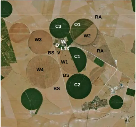
Fig. 1. Study area and fields codes.

2 Data

2.1 The study site

The test site is located in the agricultural area of Barrax (39◦30N, 2◦60W, 700 m a.s.l) near Albacete in Spain. This area is characterized by a patchwork of irrigated and non irrigated fields with different shape and size where about 65% of cultivated lands are dryland (67% winter cereals, 33% fallow) and 35% irrigated land (75% corn, 15% bar-ley/sunflower, 5% alfalfa, 5% onions and other vegetables). This area was selected as a test site for a field campaign during June–July 2005 in the framework of the international project SEN2FLEX. In Fig. 1 a map of the study area is pre-sented with the plots where ground measurements are per-formed. This area has a Mediterranean climate with dry summer and high temperatures. Distributed soil moisture measurements were made during the field campaign in the different type of vegetated fields and bare soil by University of Naples (SEN2FLEX Final Report, 2006) and these values are used as initial condition for the modeling simulation. 2.2 Land surface temperature retrieved from AHS

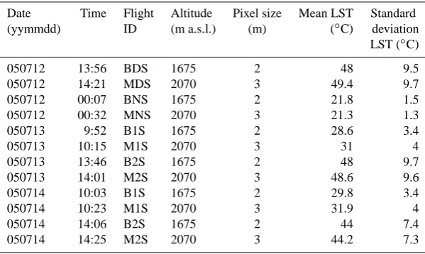
During the field campaign 12 day and night overpasses of the airplane with on board AHS were performed and images with different spatial scale resolutions (2 m and 3 m) have been collected (Table 1). Land surface temperature values are obtained with TES method (Gillespie et al., 1998) and these results are reported in (Sobrino et al., 2008).

Table 1. LST computed from AHS images.

Date Time Flight Altitude Pixel size Mean LST Standard (yymmdd) ID (m a.s.l.) (m) (◦C) deviation

LST (◦C)

050712 13:56 BDS 1675 2 48 9.5

050712 14:21 MDS 2070 3 49.4 9.7

050712 00:07 BNS 1675 2 21.8 1.5

050712 00:32 MNS 2070 3 21.3 1.3

050713 9:52 B1S 1675 2 28.6 3.4

050713 10:15 M1S 2070 3 31 4

050713 13:46 B2S 1675 2 48 9.7

050713 14:01 M2S 2070 3 48.6 9.6

050714 10:03 B1S 1675 2 29.8 3.4

050714 10:23 M1S 2070 3 31.9 4

050714 14:06 B2S 1675 2 44 7.4

050714 14:25 M2S 2070 3 44.2 7.3

is clearly visible during the day, when standard deviation of LST can reach very high values till 9.7◦C, while during the night the area seems to be homogeneous with a maximum standard deviation of 1.3◦C (Table 1).

2.3 MODIS images

LST products from MODIS radiometer on board of TERRA satellite (http://ladsweb.nascom.nasa.gov/index.html), with a spatial resolution of 1 Km, are used in this study to under-stand the ability of low resolution images from operative satellite to reproduce land surface temperature variability. A nighttime image for 13 July at 00:10 and a daytime image for 13 July at 13:45 were selected.

2.4 Thermal radiometric field campaign

Thermal radiometric ground measurements were collected by UGC – Universitad de Valencia during the airplane over-passes, during night and day, over corn (as C1 field), bare soil (BS), green grass (L13), water body (WB), wheat (as W1 field), vineyard (V), onion (O) and area of reforestation (RA) (Fig. 1). Various instruments were used to measure in the TIR domain, including multiband and single-band ra-diometers with a fixed field-of-view (Sobrino et al., 2008). 2.5 Micrometeorological stations

An eddy correlation tower in the vineyard field (V) measured the turbulent fluxes of sensible and latent heat and CO2fluxes above the canopy through the covariance between the vertical wind velocity and respectively the air temperature, the water vapour density and CO2density. Moreover relative humid-ity, air temperature, soil heat flux, soil temperature and the four component radiation were measured. The systems were installed at 410 cm height. The used energy fluxes were

col-lected from 10 July to 15 July 2005 from the Faculty of Geo-Information Science and Earth Observation of the University of Twente (SEN2FLEX Final Report, 2006; Su et al., 2008). Moreover the University of Castilla-La Mancha operated three agro-meteorological stations in the area providing me-teorological information (SEN2FLEX Final Report, 2006).

3 Hydrological model: FEST-EWB

FEST-EWB (Flash-flood Event-based Spatially-distributed rainfall-runoff Transformation-Energy Water Balance) is a distributed hydrological energy water balance model (Cor-bari et al., 2008; Cor(Cor-bari et al., 2010) and it is developed starting from the FEST-WB and the event based models FEST98 and FEST04 (Mancini, 1990; Rabuffetti et al., 2008; Ravazzani et al., 2008). FEST-EWB computes the main pro-cesses of the hydrological cycle in every cells: evapotran-spiration, infiltration, surface runoff, flow routing, subsur-face flow and snow dynamic (Corbari et al., 2009). The en-ergy balance is solved looking for the representative thermo-dynamic equilibrium temperature (RET) defined as the land surface temperature that closes the energy balance equation. So using this approach, soil moisture is linked to latent heat flux and then to LST. RET thermodynamic approach solves most of the problems of the actual evapotranspiration and soil moisture computation. In fact it permits to avoid computing the effective evapotranspiration as an empirical fraction of the potential one.

The complete energy balance equation at the ground sur-face in FEST-EWB is expressed as:

-50 0 50 100 150 200 250 300 350 400

191 193 195 197

days

L

a

ten

t Heat (W

/m 2 ) LE-fest-ewb LE-eddy station -100 -50 0 50 100 150 200 250 300

191 193 195 197

days Sens ible H e at (W /m 2 ) H-fest-ewb H-eddy station -200 -100 0 100 200 300 400 500 600 700 800

191 193 195 197

days Net r a d iat io n ( W /m 2 ) Rn-eddy station Rn-fest-ewb -100 -50 0 50 100 150

191 193 195 197

days Soi l gr ou nd f lux ( W /m 2 ) G-eddy station G-fest-ewb -50 0 50 100 150 200 250 300 350 400

191 193 195 197

days

L

a

ten

t Heat (W

/m 2 ) LE-fest-ewb LE-eddy station -100 -50 0 50 100 150 200 250 300

191 193 195 197

days Sens ible H e at (W /m 2 ) H-fest-ewb H-eddy station -200 -100 0 100 200 300 400 500 600 700 800

191 193 195 197

days Net r a d iat io n ( W /m 2 ) Rn-eddy station Rn-fest-ewb -100 -50 0 50 100 150

191 193 195 197

days Soi l gr ou nd f lux ( W /m 2 ) G-eddy station G-fest-ewb -50 0 50 100 150 200 250 300 350 400

191 193 195 197

days

L

a

ten

t Heat (W

/m 2 ) LE-fest-ewb LE-eddy station -100 -50 0 50 100 150 200 250 300

191 193 195 197

days Sens ible H e at (W /m 2 ) H-fest-ewb H-eddy station -200 -100 0 100 200 300 400 500 600 700 800

191 193 195 197

days Net r a d iat io n ( W /m 2 ) Rn-eddy station Rn-fest-ewb -100 -50 0 50 100 150

191 193 195 197

days Soi l gr ou nd f lux ( W /m 2 ) G-eddy station G-fest-ewb -50 0 50 100 150 200 250 300 350 400

191 193 195 197

days

L

a

ten

t Heat (W

/m 2 ) LE-fest-ewb LE-eddy station -100 -50 0 50 100 150 200 250 300

191 193 195 197

days Sens ible H e at (W /m 2 ) H-fest-ewb H-eddy station -200 -100 0 100 200 300 400 500 600 700 800

191 193 195 197

days Net r a d iat io n ( W /m 2 ) Rn-eddy station Rn-fest-ewb -100 -50 0 50 100 150

191 193 195 197

days Soi l gr ou nd f lux ( W /m 2 ) G-eddy station G-fest-ewb

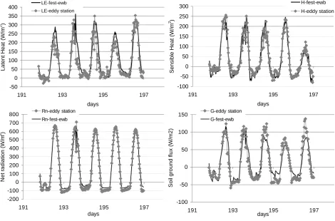
Fig. 2. Comparison between simulated and measured energy fluxes.

are respectively the sensible heat and latent heat fluxes for bare soil (s) and for canopy (c) and the energy storage terms: the photosynthesis flux (FCO2), the crop and air enthalpy changes (ScanopyandSair)and the soil surface layer heat flux (Ss)(Wm−2). These terms are often negligible, especially at basin scale with a low spatial resolution; instead at local scale the contribution of these terms could be significant (Corbari et al., 2010; Meyers and Hollinger, 2004).

FEST-EWB model is run at two different spatial resolu-tions, of 10 m and of 1000 m, for the comparison with air-borne and satellite data.

4 Energy water balance model validation

4.1 Comparison with energy fluxes from eddy covariance station

The closure of energy budget with fluxes measured at the eddy covariance station is checked to evaluate the goodness of measured ground data and the implication that has on the interpretation of energy fluxes (Wilson et al., 2002; Corbari, 2010). The closure of the energy balance with raw data shows a linear regression forced through the origin equal toy= 0.773 x with R2= 0.946 (SEN2FLEX Final Report, 2006; Su et al., 2008). Only daytime data are used for this

comparison due to problems in turbulent fluxes retrieval dur-ing stable atmospheric conditions which are typical of night (Wilson et al., 2002). Measured net radiation, latent and sen-sible heat fluxes and soil heat flux are then compared with simulated fluxes from FEST-EWB simulation at 10 m spatial resolution and a good accuracy is reached showing high val-ues of the slope of the linear regressions between measured and simulated fluxes (Fig. 2).

The goodness of these results is also confirmed from a statistical analysis looking for the minimization of the root mean square error and the maximization of the efficiency of the Nash and Sutcliffe index (Nash and Sutcliffe, 1970). Net radiation is the flux with the highest efficiency, η equal to 0.99, and the lowest RMSE, equal to 30 W/m2; instead the latent heat flux has the lowestηequal to 0.78 and the highest RMSE equal to 44.4 W/m2(Table 2).

4.2 Comparison with LST from AHS airborne radiometer

Table 2. Nash and Sutcliffe index and RMSE for the energy fluxes.

η RMSE (Wm−2) Net Radiation 0.99 30

Latent Heat 0.78 44.4 Sensible Heat 0.89 27.8 Ground Heat 0.88 17.9

reported showing a good behaviour of the model in repre-senting observed data. In particular, at this fine resolution, the model as well as the AHS is capable in representing the heterogeneity of the area that is strictly linked to vegetation type, growth vegetation period and irrigation. The mean dif-ference between RET minus LST from AHS has its maxi-mum value during the night and is equal to−1.24◦C with a standard deviation of 0.73◦C and a rout mean square error of 3.36◦C. If all 12 images are considered the total mean of the mean differences of LSTs is equal to−0.33◦C with a stan-dard deviation of 1.26◦C; but when the daytime values are compared, a mean value of−0.15◦C is reached.

4.3 Comparison with LST from ground radiometers

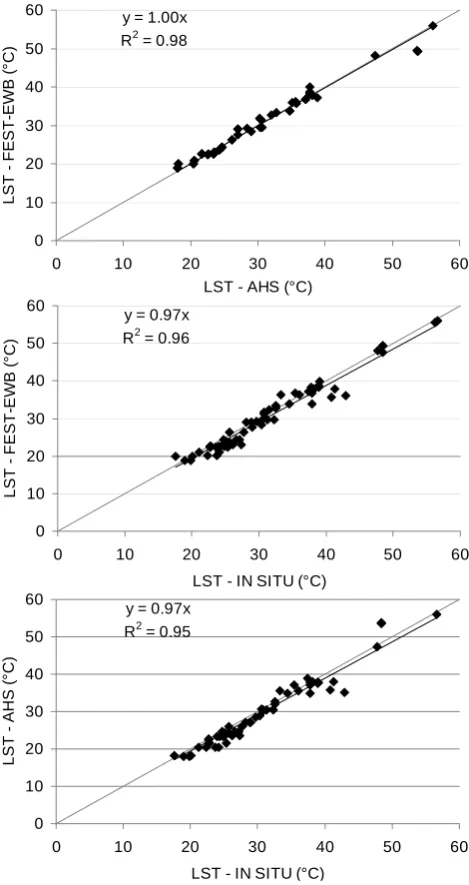
Daytime thermal infrared radiometric ground measurements are compared with land surface temperature retrieved from AHS and with simulated RET for different types of crops. Considering all the data set, good results are found (Fig. 3) with low values ofR2and of the slope of the linear regres-sion between the different temperatures. In fact the mean difference between RET and in situ measurements is equal to−1◦C with a standard deviation of 1.9◦C and RMSE of 2.1◦C. If in situ measurements and LST from AHS are com-pared, the mean difference is equal to 0.9◦C, (standard de-viation = 2.1◦C and RMSE = 2.3◦C). Good results are also found comparing RET and LST from AHS with a mean dif-ference of−0.2◦C and a standard deviation of 1.2◦C and RMSE = 1.2◦C.

5 Effect of the scale of resolution on LST spatial variability

Usually the finer the spatial scale of LST information is, the more accurate the estimate of energy and water fluxes will be. In this article the effect of the scale of resolution on LST spa-tial variability is studied. In particular LST maps from AHS and from MODIS and RET from FEST-EWB are compared for two different dates, during daytime and nighttime, to un-derstand the effect of scale resolution on land surface temper-ature variability. Spatial resolution at increasing scale offers the possibility to understand the ability of MODIS resolution to represent land surface temperature over extremely hetero-geneous area (Kustas et al., 2004; McCabe and Wood, 2006).

y = 1.00x R2 = 0.98

0 10 20 30 40 50 60

0 10 20 30 40 50 60

LST - AHS (°C)

L S T FE ST-E W B ( °C )

y = 0.97x R2 = 0.96

0 10 20 30 40 50 60

0 10 20 30 40 50 60

LST - IN SITU (°C)

L S T - F E S T -E W B (° C )

y = 0.97x R2 = 0.95

0 10 20 30 40 50 60

0 10 20 30 40 50 60

LST - IN SITU (°C)

LS T A H S ( °C )

y = 1.00x R2 = 0.98

0 10 20 30 40 50 60

0 10 20 30 40 50 60

LST - AHS (°C)

L S T FE ST-E W B ( °C )

y = 0.97x R2 = 0.96

0 10 20 30 40 50 60

0 10 20 30 40 50 60

LST - IN SITU (°C)

L S T - F E S T -E W B (° C )

y = 0.97x R2 = 0.95

0 10 20 30 40 50 60

0 10 20 30 40 50 60

LST - IN SITU (°C)

LS T A H S ( °C )

y = 1.00x R2 = 0.98

0 10 20 30 40 50 60

0 10 20 30 40 50 60

LST - AHS (°C)

L S T FE ST-E W B ( °C )

y = 0.97x R2 = 0.96

0 10 20 30 40 50 60

0 10 20 30 40 50 60

LST - IN SITU (°C)

L S T - F E S T -E W B (° C )

y = 0.97x R2 = 0.95

0 10 20 30 40 50 60

0 10 20 30 40 50 60

LST - IN SITU (°C)

LS T A H S ( °C )

Fig. 3. Scatter plots between LST from AHS, FEST-EWB and in situ measurements.

5.1 Daytime hours

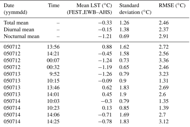
Table 3. Mean difference, standard deviation and RMSE between LST-AHS and FEST-EWB.

Date Time Mean LST (◦C) Standard RMSE (◦C) (yymmdd) (FEST EWB–AHS) deviation (◦C)

Total mean – −0.33 1.26 2.46

Diurnal mean – −0.15 1.38 2.37

Nocturnal mean – −1.21 0.69 2.91

050712 13:56 0.88 1.62 2.72

050712 14:21 −0.45 1.58 2.56

050712 00:07 −1.24 0.73 3.36

050712 00:32 −1.19 0.65 2.46

050713 9:52 −1.26 0.79 3.23

050713 10:15 −0.09 0.9 1.31

050713 13:46 0.62 1.83 2.69

050713 14:01 0.45 1.9 2.6

050714 10:03 −0.3 0.79 1.35

050714 10:23 0.13 0.85 1.39

050714 14:06 −0.71 1.69 2.7

050714 14:25 −0.78 1.83 3.12

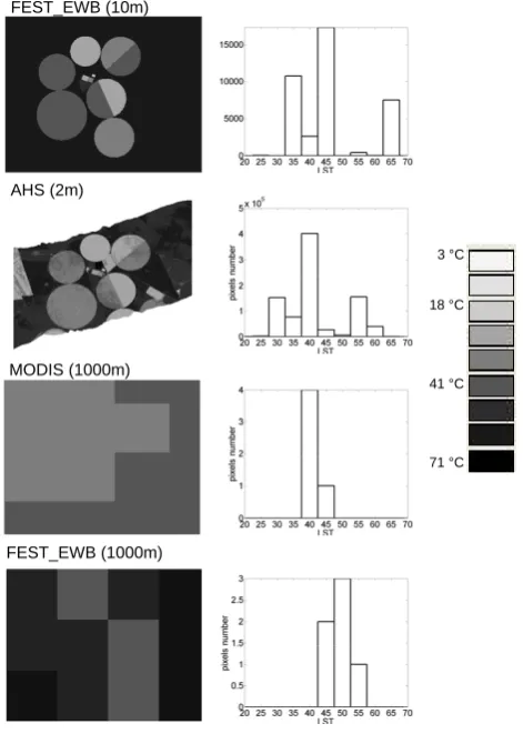
Table 4. Mean and standard deviation for the comparison between LST from MODIS, AHS and FEST-EWB.

AHS FEST-EWB FEST-EWB MODIS

(10 m) (1000 m)

13 July at 00:10

Pixel n◦ 857229 38298 6 3

Mean LST (◦C) 21 19.9 20.1 19.7

St. Dev. (◦C) 1.4 0.9 0.7 0.1

13 July at 13:46

Pixel n◦ 967450 38698 6 5

Mean LST (◦C) 42 42.9 43.8 41.3

St. Dev. (◦C) 8.8 9.6 3 1.2

Instead if MODIS LST coarser image (1000 m) and RET at the spatial resolution of 1000 m are considered, in Fig. 4 it is clearly visible that they do not capture the strong spatial heterogeneity of LST from AHS, but only the mean value (Table 4). The lower spatial accuracy of MODIS and FEST-EWB (1000 m) is also evident in the frequency distribution graphs (Fig. 4).

5.2 Nocturnal hours

The night images of 13 July at 00:10 are selected for the com-parison and a strong homogeneity in land surface tempera-ture distribution for all the three different spatial resolutions is shown (Fig. 5). In fact the difference between crops and bare soil is no longer visible, as well as the different stages

of vegetation growth and the different soil moisture condi-tions. In particular a good behaviour of FEST-EWB model in representing LST image from AHS is shown with simi-lar statistic values (Table 4). Moreover, during night time, also MODIS and FEST-EWB (1000 m) coarser images can represent this homogeneous thermodynamic characteristic of the area as well as the high resolution images (Fig. 5). In fact the four images have a similar mean value, ranging from 19.7◦C to 21◦C, and small standard deviations (from 0.1◦C to 1.4◦C) (Table 4).

Moreover, this homogeneity is also confirmed from the frequency distribution graphs (Fig. 5) where, as expected, mean values of the three images are in the same class and a low variance is found.

6 LST aggregation effect and its spatial correlation

Modelled RET and LST from AHS have been aggregated at subsequent increasing spatial resolution (50 m, 100 m, 500 m and 1000 m), keeping the same number of pixels of the 10 m image (Fig. 6), to understand their spatial variability and the aggregation effect on some statistical parameters, such as the mean, the variance and the variation coefficient (CV).

An interesting aspect of the spatial variability of land sur-face temperature at different spatial scales is the analysis of the mutual relationship between its values in each pixel. These relationships between different LST pixel values at a define distance have been analysed with the spatial autocor-relation function (AC):

AC d1,2=

E{[LST (X1)−µ]·[LST (X2)−µ]}

FEST_EWB (10m)

AHS (2m)

MODIS (1000m)

FEST_EWB (1000m)

3 °C

41 °C

71 °C 18 °C

Fig. 4. Frequency distribution for LST from AHS, FEST-EWB (10 m–1000 m) and MODIS for 13 July at 13:45.

whereµ is the mean andσ2is the variance of LST in sta-tionary hypothesis, so that a stochastic process, whose joint probability distribution does not change in time or space, is considered.x1andx2are the generic positions at a fixed dis-tance d. The autocorrelation function has been studied under isotropy hypothesis so thatdis a function only of the distance between two points and not of the direction.

LST map of 13 July 2005 at 13:46 was selected for this analysis. In Fig. 7 AC values are reported as a function of distance for RET and LST from AHS at 10 m spatial resolu-tion. The two autocorrelation functions are similar till 150 m of distance, showing the good behaviour of the model in rep-resenting the observed data at high spatial resolution. More-over, as expected, AC values are equal to 1 at a 0 m distance and decreases till values near zero as the distance between the two pixels increases. The simulation has been stopped at 560 m distance, because higher distances are of lower inter-est due to the scarce number of couples of LST points. This result implies that the presence of bare soil or of different vegetation types at different growth stages and the different soil moisture conditions are responsible of the relationship between pixels at different land surface temperatures.

FEST_EWB (10m)

AHS (2m)

MODIS (1000m)

FEST_EWB (1000m)

3 °C

41 °C

71 °C 18 °C

Fig. 5. Frequency distribution for LST from AHS, FEST-EWB (10 m–1000 m) and MODIS for 13 July at 00:10.

FEST-EWB

AHS

Fig. 6. RET from FEST-EWB (on top) and LST from AHS (below) at the different spatial resolutions of 10 m, 50 m, 100 m, 500 m and 1000 m.

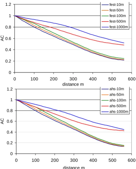
The autocorrelation functions are also reported for the dif-ferent aggregation scales for FEST-EWB and AHS and sim-ilar results are obtained. Moreover, AC values decrease with the distance but more slowly at a lower spatial resolution, due to the increasing homogeneity of the area (Fig. 8).

0 0.2 0.4 0.6 0.8 1 1.2

0 100 200 300 400 500 600

distance m

AC

FEST-EWB (10m) AHS (10m)

Fig. 7. Autocorrelation function for LST maps from FEST-EWB and AHS for 13 July 2005 at 13:46 at 10 m of spatial resolution.

0 0.2 0.4 0.6 0.8 1 1.2

0 100 200 300 400 500 600

distance m

AC

fest-10m fest-50m fest-100m fest-500m fest-1000m

0 0.2 0.4 0.6 0.8 1 1.2

0 100 200 300 400 500 600

distance m

AC

ahs-10m ahs-50m ahs-100m ahs-500m ahs-1000m

0 0.2 0.4 0.6 0.8 1 1.2

0 100 200 300 400 500 600

distance m

AC

fest-10m fest-50m fest-100m fest-500m fest-1000m

0 0.2 0.4 0.6 0.8 1 1.2

0 100 200 300 400 500 600

distance m

AC

ahs-10m ahs-50m ahs-100m ahs-500m ahs-1000m

Fig. 8. Comparison between autocorrelation functions for LST maps from FEST-EWB model at different spatial resolution of 10 m, 50 m, 100 m, 500 m and 1000 m.

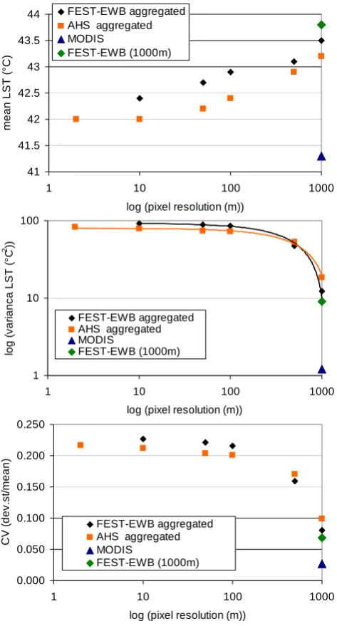
The more common statistical parameters have also been analysed and, as expected, variances and CVs decrease with increasing the aggregation area, while the mean val-ues remain almost constant (Rodriguez-Iturbe et al., 1995) (Fig. 10). In particular the variances can be interpolated as two power law functions and the passage between them seems to be located at the autocorrelation distance, equal about to 500 m. This means that with the increase of the

ag-0 0.2 0.4 0.6 0.8 1 1.2

0 100 200 300 400 500 600

distance m

AC

FEST-EWB aggregated (1000m) AHS aggregated (1000m) MODIS

FEST-EWB (1000m)

Fig. 9. Comparison between autocorrelation functions of LST from MODIS, FEST-EWB and AHS at the spatial resolution of 1000 m.

gregation area further than the autocorrelation distance, pix-els with higher difference of LST are included into the aggre-gation area. AHS and FEST-EWB aggregated images seem to have a similar behaviour during this aggregation process; instead, if the statistical parameters for LST from MODIS and FEST-EWB simulated at 1000 m are considered, lower values of variance and variation coefficient in comparison to the ones of the aggregated FEST-EWB and AHS at 1000 m are found.

6.1 LST scale of fluctuation

In the analysis of signal, the concept of scale of fluctuation (VanMarcke, 1983) can be used as a significant parameter to understand the spatial variability of a generic process. This theory will be used to characterize land surface temperature from FEST-EWB and from AHS.

In particular for a stationary process, the scale of fluctua-tion can be defined as:

α=lim0(A)·A

A−→∞

(3) where0(A)=σ_A2/σ2,Ais the aggregation area andσ_A2is the variance of the aggregated process.

0(A) is linked to the correlation function as:

0(A)= 1

L1L2

L1

Z

−L2

L2

Z

−L1

(1−|d1|

L1

)(1−|d2|

L2

)AC(d1,2)·d1·d2 (4)

So the scale of fluctuation can also be expressed as func-tion of the correlafunc-tion funcfunc-tion, as the volume below the AC function:

α=

L1

Z

−L2

L2

Z

−L1

AC(d1,2)·d1·d2 (5)

if this hypothesis is verified: lim AC(d1,2)=0

d1,2−→∞

41 41.5 42 42.5 43 43.5 44

1 10 100 1000

log (pixel resolution (m))

me a n L S T ( °C ) FEST-EWB aggregated AHS aggregated MODIS

FEST-EWB (1000m)

1 10 100

1 10 100 1000

log (pixel resolution (m))

lo g ( v a ri a nca L S T ( °C 2)) FEST-EWB aggregated AHS aggregated MODIS FEST-EWB (1000m) 0.000 0.050 0.100 0.150 0.200 0.250

1 10 100 1000

log (pixel resolution (m))

C V (d e v .s t/m e a n ) FEST-EWB aggregated AHS aggregated MODIS FEST-EWB (1000m) 41 41.5 42 42.5 43 43.5 44

1 10 100 1000

log (pixel resolution (m))

me a n L S T ( °C ) FEST-EWB aggregated AHS aggregated MODIS

FEST-EWB (1000m)

1 10 100

1 10 100 1000

log (pixel resolution (m))

lo g ( v a ri a nca L S T ( °C 2 )) FEST-EWB aggregated AHS aggregated MODIS FEST-EWB (1000m) 0.000 0.050 0.100 0.150 0.200 0.250

1 10 100 1000

log (pixel resolution (m))

C V (d e v .s t/m e a n ) FEST-EWB aggregated AHS aggregated MODIS FEST-EWB (1000m) 41 41.5 42 42.5 43 43.5 44

1 10 100 1000

log (pixel resolution (m))

me a n L S T ( °C ) FEST-EWB aggregated AHS aggregated MODIS

FEST-EWB (1000m)

1 10 100

1 10 100 1000

log (pixel resolution (m))

lo g ( v a ri a nca L S T ( °C 2)) FEST-EWB aggregated AHS aggregated MODIS FEST-EWB (1000m) 0.000 0.050 0.100 0.150 0.200 0.250

1 10 100 1000

log (pixel resolution (m))

C V (d e v .s t/m e a n ) FEST-EWB aggregated AHS aggregated MODIS

FEST-EWB (1000m)

Fig. 10. Comparison between the mean, the standard deviation and the variation coefficient for LST from AHS and FEST-EWB at dif-ferent spatial resolution (10 m, 50 m, 100 m, 500 m and 1000 m) and LST from MODIS and FEST-EWB simulated at 1000 m.

Due to the fact that at different aggregation level an auto-correlation function exists (Fig. 8), a scale function can be defined for each spatial resolution, but only starting from the highest resolution to the lowest one and not viceversa. In this wayαcan be used as a superior limit above which continu-ing the aggregation process, the information about variance are lost.

The scale of fluctuation can be also written in the fre-quency field:

α=4π2·g(0,0) (7)

0 5 10 15 20 25

0.00E+00 2.00E+05 4.00E+05 6.00E+05 8.00E+05 1.00E+06 1.20E+06

aggregation area (m2)

α

(

m2

) FEST-EWB

AHS

Fig. 11. Scales of fluctuation of LST for different aggregation areas.

whereg(ω1ω2)is the spectral density functionG(ω1ω2) di-vided by the variance at the scale of the process andω1ω2are the frequencies in the directiond1andd2. The spectral den-sity function is the Fourier transform of the autocorrelation AC function.

In Fig. 11 the scales of fluctuation for RET and LST from AHS are reported andαgrows with the growing of the ag-gregation area very quickly, but for A >> α the scales of fluctuation remain constant. This constant value, from the definition of scale of fluctuation, is the estimate of the area above which LST variance becomes insignificant for the pro-cess. These results confirm the previous ones, showing that the area of significance of this hydrological variable is equal to the area defined from the autocorrelation function.

From these analyses, for a process at higher aggregation, the variance tends to zero while the scale of fluctuation is higher. So that the product between the scale of fluctuation and the relative variance is constant:

αa·σa2=αA·σA2 (8)

These concepts can also be related to the hydrological mod-elling observing that a lumped model has obviously a bigger level of indetermination than a distributed model.

7 Conclusions

The representativeness of LST for a distributed hydrological water balance model, FEST-EWB, has been analysed. The hydrological model performed well for the whole period of observation and was able to accurately predict energy fluxes measured at an eddy covariance station and land surface tem-perature spatial and temporal distribution in comparison to in situ thermal infrared radiometric measurements, high and low spatial resolution remote sensing images.

with high standard deviation. On the contrary, MODIS im-ages, due to the low spatial resolution, are able to detect only the mean LST value. Instead during night time, coarser im-ages spatial resolution seems to be sufficient to represent the lower LST spatial variability of the fields showing the same statistics of higher resolution images. This observation high-lights the role of operative satellite that can be used in an as-similation process into hydrological energy balance models. Moreover AHS and FEST-EWB aggregated images seem to have a similar behaviour during the aggregation process showing similar values of variance, CV and autocorrelation function; while the coarser LST from MODIS and FEST-EWB simulated at 1000m have lower values of variance and variation coefficient.

A constant value of the scale of fluctuation, above which LST variance becomes insignificant for the process, is reached and it is equal to the significant area found from the autocorrelation function.

Acknowledgements. This work was funded by MIUR in the

framework of the Azioni Integrate Italia-Spagna project (prot. IT09G9BLE4) “Land Surface temperature from remote sensing for operative validation of an hydrologic energy water balance model” and of the ACQWA EU/FP7 project (grant number 212250) “Assessing Climate impacts on the Quantity and quality of WAter”.

Edited by: D. F. Prieto

References

Anderson, M. C., Norman, J. M., Mecikalski, J. R., Torn, R. D., Kustas, W. P., and Basara, J. B.: A multiscale remote sensing model for disaggregating regional fluxes to micrometeorological scales, J. Hydrometeorol., 5, 343–363, 2004.

Bastiaanssen, W. G. M., Menenti, M., Feddes, R. A., and Holtslag, A. A. M.: A remote sensing surface energy balance algorithm for land (SEBAL) 1. Formulation, J. Hydrol., 212–213, 198–212, 1998.

Bl¨oschl, G. and Sivapalan, M.: Scale issues in hydrological mod-elling: a review, Hydrol. Processes, 9(3–4), 251–290, 1995. Corbari, C., Horeschi, D., Ravazzani, G., and Mancini, M.:

Land surface temperature from remote sensing and energy water balance model for irrigation management, Options M´editerran´eennes, A84, 223–234, 2008.

Corbari, C., Ravazzani, G., Martinelli, J., and Mancini, M.: Eleva-tion based correcEleva-tion of snow coverage retrieved from satellite images to improve model calibration, Hydrol. Earth Syst. Sci., 13, 639–649, doi:10.5194/hess-13-639-2009, 2009

Corbari C.: Energy water balance and land surface temperature from satellite data for evapotranspiration control. PhD disserta-tion, Politecnico di Milano, Milan, Italy, 2010.

Dooge, J. C. I.: Looking for hydrologic laws, Water Resour. Res., 22(9) 46S–58S, 1986.

Famiglietti J. S. and Wood E. F.: Multiscale modelling of spatially variable water and energy balance processes, Water Resour. Res., 30, 3061–3078, 1994.

Giacomelli A., Bacchiega, U., Troch, P. A., and Mancini, M.: Eval-uation of surface soil moisture distribution by means of SAR re-mote sensing techniques and conceptual hydrological modelling, J. Hydrol., 166, 445–459, 1995.

Gillespie, A., Rokugawa, S., Matsunaga, T., Cothern, J. S., Hook, S., and Kahle, A. B.: A temperature and emissivity separation algorithm for advanced spaceborne thermal emission and reflec-tion radiometer (ASTER) images, Ieee T. Geosci. Remote, 36, 1113–1126, 1998.

Jasper, K., Gurtz, J., and Lang, H., Advanced flood forecasting in Alpine watershed by coupling meteorological and forecasts with a distributed hydrological model, J. Hydrol, 267, 40–52, 2002. Jim´enez-Mu˜noz, J. C. and Sobrino, J. A.: Feasibility of

retriev-ing land surface temperature from ASTER TIR bands usretriev-ing two-channel algorithms: a case study of agricultural areas, Ieee Geosci. Remote S., 4(1), 60–64, 2007.

Kustas, W. P., Li, F., Jackson, T. J., Prueger, J. H., MacPherson, J. I., and Wolde, M.: Effects of remote sensing pixel resolution on modelled energy flux variability of croplands in Iowa, Remote Sens. Environ., 92(4), 535–547, 2004.

Mancini, M.: La modellazione distribuita della risposta idrologica: effetti della variabilit`a spaziale e della scala di rappresentazione del fenomeno dell’assorbimento. PhD dissertation, Politecnico di Milano, Milan, Italy , 1990 (in italian).

Mancini, M., Hoeben, R., and Troch, P.: Multifrequency Radar Ob-servations of Bare Surface Soil Moisture Content: A Laboratory Experiment, Water Resour. Res., 35(6), 1827–1838, 1999. McCabe, M. F. and Wood, E. F.: Scale influences on the remote

estimation of evapotranspiration using multiple satellite sensors, Remote Sens. Environ., 105, 271–285, 2006.

Meyers T. P. and Hollinger S. E.: An assessment of storage terms in the surface energy balance of maize and soybean, Agr. Forest Meteorol., 125, 105–115, 2004.

Minacapilli, M., Agnese, C., Blanda, F., Cammalleri, C., Ciraolo, G., D’Urso, G., Iovino, M., Pumo, D., Provenzano, G., and Rallo, G.: Estimation of actual evapotranspiration of Mediter-ranean perennial crops by means of remote-sensing based surface energy balance models, Hydrol. Earth Syst. Sci., 13, 1061–1074, doi:10.5194/hess-13-1061-2009, 2009.

Montaldo N. and Albertson, J. D.: On The Use Of The Force-Restore SVAT Model Formulation For Stratified Soils, J. Hy-drometeorol., 2(6), 571–578, 2001.

Montaldo, N., Ravazzani G., and Mancini, M.: On the prediction of the Toce alpine basin floods with distributed hydrologic models, Hydrol. Processes, 21, 608–621, 2007.

Nash J. E. and Sutcliffe J. V.: River flow forecasting through the conceptual models, Part 1: A discussion of principles, J. Hydrol., 10(3), 282–290, 1970.

Noihlan J. and Planton S.: A Simple parameterization of Land Sur-face Processes for Meteorological Models, Mon. Wea. Rev., 117, 536–549, 1989.

Norman, J. M., Kustas, W. P., and Humes, K. S.: Source approach for estimating soil and vegetation energy fluxes in observations of directional radiometric surface temperature, Agr. Forest Me-teorol., 77, 263–293, 1995.

doi:10.5194/nhess-8-161-2008, 2008.

Ravazzani, G., Rabuffetti, D., Corbari, C., and Mancini, M.: Valida-tion of FEST-WB, a continuous water balance distributed model for flood simulation, Proceedings of XXXI Italian Hydraulic and Hydraulic Construction Symposium, Perugia, Italy, 2008. Rodriguez-Iturbe, I., Vogel, G. K., Rigon, R., Entekhabi, D.,

Castelli, F., and Rinaldo, A.: On the spatial organization of soil misture fields, Geophys. Res. Lett., 22(20), 2757–2760, 1995. Schmugge T. J., Kustas W. P., and Humes K. S.: Monitoring Land

Surface Fluxes Using ASTER Observations Ieee, T. Geosci. Re-mote, 36(5), 1998.

SEN2FLEX Final Report (Contract no:19187/05/I-EC 17628/03/NL/CB 17336/03/NL/CB), in: Proceedings of the SPARC, 4–5 July 2006, Enschede, ESA Publications Division, Noordwijk, The Netherlands.

Sivaplan, M. and Wood, E. F.: Spatial Heterogeneity and Scale in the Infiltration Response of Catchments Scale Problems in Hy-drology: Runoff Generation and Basin Response, D. Reidel Pub-lishing Co., Dordrecht Holland, NSF Grant No. CEE-8100491 and NASA Grant No. NAG-5/491, 81–106, 1986.

Sobrino J. A., Li, Z. L., Stoll, M. P., and Becker, F.: Improvements in the split-window technique for land surface temperature deter-mination, Ieee T. Geosci. Remote, 32(2), 243–253, 1994. Sobrino, J. A., Jim´enez-Mu˜noz, J. C., S`oria, G., G´omez, M., Ortiz,

A. Barella, Romaguera, M., Zaragoza, M., Julien, Y., Cuenca, J., Atitar, M., Hidalgo, V., Franch, B., Mattar, C., Ruescas, A., Morales, L., Gillespie, A., Balick, L., Su, Z., Nerry, F., Peres, L., and Libonati, R.: Thermal remote sensing in the framework of the SEN2FLEX project: field measurements, airborne data and applications, Int. J. Remote Sens., 29(17), 4961–4991, 2008. Soria, G. and Sobrino, J. A.: ENVISAT/AATSR derived land

sur-face temperature over a heterogeneous region, Remote Sens. En-viron., 111, 409–422, 2007.

Su, Z., Pelgrum, H., and Menenti, M.: Aggregation effects of sur-face heterogeneity in land sursur-face processes, Hydrol. Earth Syst. Sci., 3, 549–563, doi:10.5194/hess-3-549-1999, 1999.

Su, Z.: The Surface Energy Balance System (SEBS) for estima-tion of turbulent heat fluxes, Hydrol. Earth Syst. Sci., 6, 85–100, doi:10.5194/hess-6-85-2002, 2002.

Su, Z., Timmermans, W. J., Gieske, A. S. M., Jia, L., Elbers, J. A., Olioso, A., Timmermans, J., van der Velde, R., Jin, X., van der Kwast, H., Nerry, F., Sabol, D., Sobrinos, J. A., Moreno, J., and Bianchi, R.: Quantification of land atmosphere exchanges of wa-ter, energy and carbon dioxide in space and time over the hetero-geneous Barrax site, Int. J. Remote Sens., 29, 17–18, 5215–5235, 2008.

Troch, P. A., Mancini, M., Paniconi, C., and Wood, E. F.: Eval-uation of a Distributed Catchment Scale Water Balance Model, Water Resour. Res., 29(6), 1805–1817, 1993.

VanMarcke, E.: Random Fields: Analysis and Synthesis. The MIT press Cambridge Massachusetts, London, England, 1983. Wilson, K., Goldstein, A., Falge, E., Aubinet, M., Baldocchi, D.,

Berbigier, P., Bernhofer., C., Ceulemans, R., Dolman, H., Field, C., Grelle, A., Ibrom, A., Law, B. E., Kowalski, A., Meyers, T., Moncrieff, J., Monson, R., Oechel, W., Tenhunen, J., Valentini, R., and Verma, S.: Energy balance closure at FLUXNET sites, Agr. Forest Meteorol., 113, 223–243, 2002.

Wood, E. F., Sivapalan, M., Beven, K., and Band, L.: Effects of spatial variability and scale with implications to hydrologic mod-elling, J. Hydrol., 102(1–4), 29–47, 1988.

Wood, E. F.: Scaling soil moisture and evapotranspiration in runoff models, Adv. Water Resour., 17, 1–2, 1994.