Corresponding author: TANG Wei (1971-), Male Doctor, Professor of Shaanxi University of Science & Technology, PhD Tutor. Research direction: Pulp and Paper Process Automation; Industrial Process Advanced Control; Large Time-delay Process Control and Application. Tel:13892980876; E-mail:[email protected]
Abstract—This paper proposes a strategy for designing pitch, yaw and supervisory control of wind turbine including a 3D modeling of the whole system. The system is considered here to avoid mechanical losses as well as maintain a constant rotor speed in wind turbine. The wind speed will be varying from time to time, so to protect the turbine from any kind of damage due to wind speed variation, the pitch control system is designed. The direction of nacelle is also varying with time to capture the maximum energy from the air, a yaw control system is premeditated. To analyze operating conditions for determining the state of turbine to enable or disable operation such as bringing the turbine to stop by applying parking brake or releasing the brake enabling the turbine to spin, supervisory control system is introduced as an intermediary link in between pitch and yaw control system to avoid undesirable events. The 3D model, pitch, yaw and supervisory control system of wind turbine has been simulated in MATLAB SimulinkTM and
simulation results also show the coherence with the proposed analogy.
Index Terms— Blade forces; Pitch, Yaw and Supervisory Control; 3D Modeling of Wind Turbine; Renewable Energy.
INTRODUCTION
ince 1979, the Chinese economy has increased at an average annual rate of 10%, doubling every 7 years. To maintain this high rate of economic growth, China needs to continue expanding its electricity supply. China is rich in coal reserves, but limited in gas and oil supply. Electricity generation based
on coal is highly polluting and carbon-intensive, thus creating significant political and international pressure [1]. As an alternative, China has so far achieved remarkable progress in wind energy development. Wind power now represents 4% of the overall power generation [2] which is largely due to the country’s vast wind resource, relative technical maturity and relatively low cost compared to other renewable resources. In 2018, China has produced 366,000 GWh [3] electricity from wind energy having the capacity of 184,260 MW [4]. To capture the maximum power from wind, after the capital costs of commissioning wind turbine generators, the biggest costs are operations, maintenance and insurance. Reducing maintenance and operating costs can considerably reduce the payback period and provide the impetus for investment and extensive acceptance of this clean energy source.
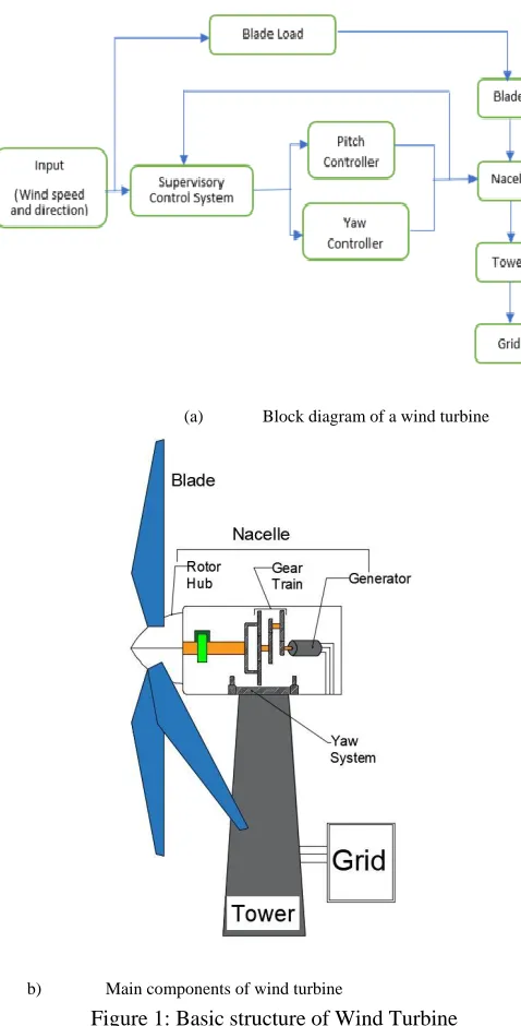
A wind turbine has a tower, in top of the tower there sits the nacelle. Inside the nacelle, we will find the generator which is connected to the electrical grid. The wind turbine attempts to spin the generator at a constant speed or at its rated speed. For the generator to spin, we have a hub which can rotate and blades are connected to the hub. The wind strikes the blades which enables the hub to rotate and the hub is connected to the generator with a gear train. In order to control the lift and drag which the blades generate, a yaw control system that points the wind turbine into the incoming wind and there is a pitch control system that controls the angle of the blades in order to control how much lift and drag the blades produce. The gearbox interconnects the rotor shaft and generator shaft. The power generated from the generator is sent to the grid by a transformer. A basic structure of wind turbine is given below in Fig. 1.
A Basic Approach for Designing Pitch, Yaw
and Supervisory Control System of Wind
Turbines
Tang Wei 1; Md. Muhie Menul Haque1, 2; Shi Yong1; Liu Yan1
College of Electrical and Information Engineering,
1Shaanxi University of Science and Technology, Xi’an, Shaanxi, 710021, PR of China.
In affiliation with 2Bangladesh University of Engineering and Technology.
DOI: 10.29322/IJSRP.9.11.2019.p9598
http://dx.doi.org/10.29322/IJSRP.9.11.2019.p9598
(a) Block diagram of a wind turbine
[image:2.612.56.295.57.527.2]b) Main components of wind turbine
Figure 1: Basic structure of Wind Turbine
The fundamental equation of wind power answers the most basic quantitative question-how much energy can be generated by a wind turbine per unit time. The power of the wind is the rate of wind energy flow through an open window. Wind energy depends on three factors- a) amount of air (the volume of air in consideration), b) speed of air (the magnitude of its velocity), c) mass of air( related to its volume via density). In other words, wind power is the rate of kinetic energy flow. Using the fluid mechanics concept, the fundamental equation in power analysis can be derived [5].
𝑃 =1
2∙ 𝜌 ∙ 𝐴 ∙ 𝑣
3 (1)
Where 𝑃 = available power of wind; 𝜌 = density of air; 𝐴 =
swept area by the wind; 𝑣 = velocity of the wind. It exhibits a highly nonlinear cubic dependency on wind speed. Wind
turbines reach the highest efficiency at a wind speed between 10 and 15 ms-1. Above this wind speed, the power output of the
rotor must be controlled to reduce driving forces on the rotor blades as well as the load on the whole wind turbine structure [6]. High winds occur only for short periods and hence have little influence in terms of energy production. All wind turbines are designed with a type of power control. There are different ways to control aerodynamic forces on the turbine rotor and therefore limit the power in high winds in order to avoid damage to the wind turbine [7].
Advanced control strategies for wind turbines have been investigated over a few decades which are broadly classified into the classic control, modern control and intelligent control [8] as shown in Table I.
Table I Classification of Wind Turbine Control Strategy
Control theory
Classical control
Modern control Intelligent control Control objective SISO, LTI system SISO/SIMO/MIS O/MIMO, Linear/nonlinear time variant/invariant/ univariate/multiv ariate, Discrete/continu ous system Large scale, Complex structure, Incomplete information, Multivariate system Analysis method Frequency domain approach Time-domain approach Time-domain approach Mathemat ical model Transfer function State-Space equation Subsystem Mathemat ical tool Laplace transform Matrix Algebra, Vector-space theory Cybernetics, Operation research, Artificial intelligence Control method PID Control Optimal Control, Robust Control, Adaptive Control, Sliding Model Control, Predictive Model Control Bayesian Control, Fuzzy Control, Neural network Control, Genetic Algorithm, Intelligent agents
[image:2.612.314.571.304.675.2]the maximum power point tracking (MPPT) is obtained. To achieve the MPPT, the classical PI controller is used which is simple and practical, but needs to tune the PI parameters repeatedly. In the full load regime, the main control objectives are to regulate both the generator power and speed at their rated values, respectively. These objectives can be achieved by manipulating the desired pitch angle and/or generator torque set-point.
Sometimes unwanted loads are caused by the wind at the blades such as sudden changes in wind direction, uneven loading of blades, wind turbulence and accumulation of dust on the blades. All these factors influence the generation rate of electric power. The basic formulation and governing equations regarding wind turbine modelling has been discussed in section 2 and 3D modeling of the whole project has been developed using various contents like Simscape multibody, Simmechanics, Simhydraulics in MATLAB. In section 3, the control schemes required for capturing maximum power from wind have been discussed named as pitch, yaw and supervisory control systems. The mechanical power of the wind turbine is controlled by the pitch angle adjustment of the blades. If the wind speed is greater than the rated wind speed, the pitching angle should be increased and if it’s lesser than rated speed, the pitching angle should be reduced. For the sudden change in wind direction, the yaw action should occur i.e. move the whole nacelle in the direction to the upcoming wind. So, a single control system with four servo motors at 900 apart from each other has been
considered which should operate simultaneously. After that, an overall supervisory control system is required to monitor the state of the turbine in case of emergency or during the time of maintenance and to identify statutory constraints of the turbine like whether its running on rated speed or not, generator becomes saturated or not etc. Different types of simulations using MATLAB are performed and results have been discussed in section 4 and 5. Simulation parameters have been given in the Appendix (Part B). Finally, the paper concludes with a generic discussion and suggestion about future scopes of work.
WIND TURBINE MODELING
[image:3.612.317.564.55.91.2]Modeling is a basic tool for analysis such as optimization, design and control. Wind energy conversion systems are very different in nature from conventional generators and therefore dynamic studies must be addressed in order to integrate wind power into the power system. Models used for steady-state analysis are extremely simple while the dynamic models for various types of analysis related to system dynamics: stability, control system and optimization. Modern wind turbine generator systems are constructed mainly as systems with a horizontal axis of rotation, a wind wheel consisting of three blades, a high speed asynchronous generator (also known as induction generator) and a gear box. Asynchronous generators are used because of their advantages, such as simplicity of construction, possibilities of operating at various operational conditions and low investment and operating costs. A typical wind energy conversion system is displayed in Fig. 2.
Figure 2: Wind turbine energy conversion scheme
B. Modeling of Blades
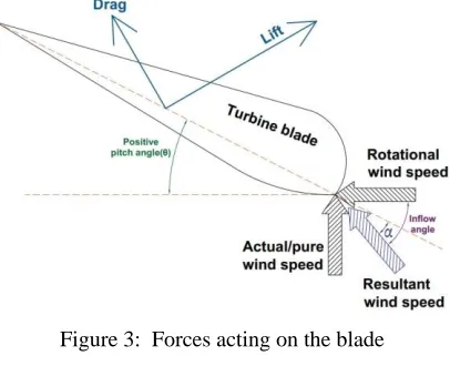
The forces that are acting on rotor blades which are generated from the wind speed during the conversion of the kinetic energy of the wind into mechanical power then converted into electrical power is described by the aerodynamic system [9]. There are mainly two forces on the blade which cause the moment in the blades, the forces are lift and drag force. The torque and thrust force are resolved from the tangential component and an axial component respectively. The forces acting on the blades are shown in Fig. 3.
Figure 3: Forces acting on the blade
Lift force =1
2∙ 𝐶𝐿∙ 𝜌 ∙ 𝐴 ∙ 𝑣
2
Drag force =1
2∙ 𝐶𝐷∙ 𝜌 ∙ 𝐴 ∙ 𝑣
2
Rotational wind speed(𝑣𝑟) = 𝑅𝑜𝑡𝑜𝑟 𝑠𝑝𝑒𝑒𝑑(𝜔) × 𝑅𝑎𝑑𝑖𝑢𝑠
Inflow angle = tan−1[ 𝐼𝑛𝑖𝑡𝑖𝑎𝑙 𝑤𝑖𝑛𝑑 𝑠𝑝𝑒𝑒𝑑(𝑣𝑖𝑛𝑡)
𝑅𝑜𝑡𝑎𝑡𝑖𝑜𝑛𝑎𝑙 𝑤𝑖𝑛𝑑 𝑠𝑝𝑒𝑒𝑑(𝑣𝑟)
]
Angle of attack(𝛼) = 𝐼𝑛𝑓𝑙𝑜𝑤 𝑎𝑛𝑔𝑙𝑒 − 𝑃𝑖𝑡𝑐ℎ 𝑎𝑛𝑔𝑙𝑒
Where,
𝐶𝐿= coefficient of lift; 𝐶𝐷
= coefficient of drag and they depend on angle of attack(𝛼)
As mentioned earlier in (1), the turbine blades extract kinetic energy in the wind and transform it into mechanical energy. The kinetic energy in air of an object of mass m moving with speed v is equal to,
𝐸 =1
2∙ 𝑚 ∙ 𝑣
2 (II.A.1)
[image:3.612.339.542.265.430.2]𝑃𝑤= 𝑑𝐸 𝑑𝑡 =
1 2∙ 𝑚 ∙ 𝑣
2 (II.A.2)
Where m is the mass flow rate per second. When the air passes across an area A (e.g. the area swept by the rotor blades), the power in the air can be computed by using (1). The air density
𝜌 can be expressed as a function of the turbine elevation above sea level H,
𝜌 = 𝜌0− 1.194 × 10⁻⁴∙ 𝐻 (II.A.3)
Where 𝜌0= 1.225 kgm−3 is the air density at sea level at temperature, 𝑇 = 298𝐾.
The power extracted from the wind is given by
𝑃𝐵𝑙𝑎𝑑𝑒= 𝐶𝑝(𝜆, 𝛽) ∙ 𝑃𝑤= 𝐶𝑝(𝜆, 𝛽) ∙ 1
2∙ 𝜌 ∙ 𝐴 ∙ 𝑣
3 (II.A.4)
The power factor, 𝐶𝑝 has a maximum theoretical value equal to 0.593 and a function of the tip-speed ratio (𝜆) and the blade pitch angle (𝛽) in degrees. The blade pitch angle is defined as the angle between the plane of rotation and the blade cross-section chord. The tip-speed ration is defined as,
𝜆 =𝜔𝑚∙𝑅
𝑣 (II.A.5)
Where 𝜔𝑚 is the angular velocity of the rotor and R is the rotor radius (blade length).
The rotor torque 𝑇𝑤 can be computed as
𝑇𝑤=𝑃𝐵𝑙𝑎𝑑𝑒
𝜔𝑚 =
𝐶𝑝(𝜆,𝛽)∙12∙𝜌∙𝐴∙𝑣3
𝜔𝑚 (II.A.6)
The power coefficient 𝐶𝑝 can be defined as a function of the tip-speed ratio and the blade pitch angle as follows:
𝐶𝑝(𝜆, 𝛽) = 𝑐1(𝑐2∙1
𝛾− 𝑐3∙ 𝛽 − 𝑐4∙ 𝛽 𝑥− 𝑐
5) 𝑒 −𝑐6∙𝛾1
(II.A.7)
With 𝛾 defined as
1 𝛾=
1 𝜆+0.08𝛽−
0.035
1+𝛽3 (II.A.8)
While the coefficients 𝑐1~𝑐6are proposed as equal to: 𝑐1= 0.5, 𝑐2= 116, 𝑐3= 0.4, 𝑐4= 0, 𝑐5= 5, 𝑐6= 21 (‘x’ is not used here as 𝑐4= 0)
[image:4.612.314.535.50.221.2]An example of the power coefficient [𝐶𝑝(𝜆, 𝛽)] characteristics computed taking into account (II.A.7, II.A.8) and the parameters 𝑐1~𝑐6 for a given rotor diameter, rotor speed and for various blade pitch angles (𝛽) is presented in Fig. 4 [10]. The 3D modeling of the blades has been given in the Appendix (Part C).
Figure 4: Analytical approximation of 𝐶𝑝(𝜆, 𝛽) characteristics
C. Modeling of Drive-train
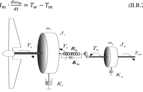
The drive train of a wind turbine system generally consists of a blade pitching mechanism, a hub with blades, a rotor shaft and a gearbox with generator. The drive train model presented in this paper includes the inertia of both the turbine and generator. The moment of inertia (MOI) of the wind wheel (hub with blades) is about 90% of the drive train total moment, while the generator rotor MOI is equal to about 10%, the generator represents the biggest torsional stiffness. The structure of the model is presented in Fig. 5 [11].
The equations of motion of the induction generator is given by
𝐻𝑔∙𝑑𝜔𝑔
𝑑𝑡 = 𝑇𝑒+
𝑇𝑚
𝑛 (II.B.1)
Since the wind turbine shaft and generator are coupled together through a gearbox, the turbine shaft system should not be considered stiff. To account for the interaction between the wind turbine and rotor, an additional equation describing the motion of the wind turbine shaft is adopted.
𝐻𝑚∙𝑑𝜔𝑚
𝑑𝑡 = 𝑇𝑤− 𝑇𝑚 (II.B.2)
[image:4.612.318.560.518.675.2]The mechanical torque 𝑇𝑚 can be modelled with the following equation,
𝑇𝑚 = 𝐾 ∙𝜃
𝑛+ 𝐷 ∙ (
𝜔𝑔−𝜔𝑚
𝑛 ) (II.B.3)
𝑑𝜃
𝑑𝑡 = 𝜔𝑔− 𝜔𝑚 (II.B.4)
Where n is the gear ratio, 𝜃 is the angle between the turbine rotor and the generator rotor; 𝜔𝑚, 𝜔𝑔, 𝐻𝑚 and 𝐻𝑔 are the turbine and generator rotor speed and inertia constant, respectively. K and D are the drive train stiffness and damping constants; 𝑇𝑤 is the torque provided by the wind (from section A) and 𝑇𝑒 is the electromagnetic torque. The 3D modeling of the gear train system has been given in the Appendix (Part C).
D. Yaw System Modeling
Yaw system plays an important role in wind turbine generator because of the direction and intensity of wind is time-varying. Yaw system consists of yaw control system and yaw drive system which mainly make the wind wheel track the wind direction and unwind the cables automatically when it is winded in a certain amount of rings [12]. The yaw movement differential equation is given below:
𝐽𝑑2𝛼
𝑑𝑡2+ 𝑘𝑎∙ 𝑑𝛼
𝑑𝑡 = 𝐹𝑣 (II.C.1)
Where 𝛼 is the yaw rotational angle; J is the nacelle inertia; ka
is the air friction constant and Fv is the wind force, as follows:
𝐹𝑣= 𝐹0cos 𝛼; 𝐹0= 𝑘𝑣∙ 𝑣2 (II.C.2)
Where 𝑘𝑣 is a constant and v is the wind velocity.
The yaw angle is the angle between the direction of the oncoming wind speed and the rotor axis and the turbine power is multiplied by the cosine of the yaw angle. When there is a non-zero yaw angle, the wind does not strike the leading edge of the blade orthogonally. Hence, the blade does not generate the same lift forces as it would generate with orthogonal inflow. Therefore, for the calculation of turbine power, only the orthogonal component of wind should be used. So, (II.A.4) can be written as [13],
𝑃𝐵𝑙𝑎𝑑𝑒= 𝐶𝑝(𝜆, 𝛽) ∙12∙ 𝜌 ∙ 𝐴 ∙ 𝑣3∙ (cos 𝛼)3 (II.C.3)
In reality, the simulation is complex. To obtain the real power that is produced by the rotor accurately, a detailed study using computational fluid dynamics (CFD) should be performed. It is beyond the scope of this work to perform such calculations.
E. Modeling of the Asynchronous Generator
The mechanical power of the wind turbine is converted into electrical power by an AC or DC generator. The AC generator can be either a synchronous or an induction (asynchronous) machine. The latter is the most widely used in wind power
industry and was selected for this project. The electrical machine works on the principle of action and reaction of electromagnetic induction. The resulting electromechanical energy conversion is reversible. As we have focused on control systems of the turbine and dynamic modeling is beyond the scope of this paper, the fixed speed induction generator has been considered which is discussed in [14], [15].
CONTROL SYSTEMS
For the proper operation of wind turbine, we have considered three control systems namely pitch, yaw and supervisory. Pitch control will help to monitor the blade position by adjusting angle of attack. Yaw control will assist to determine nacelle movement as per requirement and finally supervisory control system will govern the overall state of the turbine.
F. Blade Pitch Control System
Let us consider, the wind turbine has three blades. To control the pitch angle of the blade, hydraulic actuator is used for each blade and all the three hydraulic actuators should act simultaneously. The blade of wind turbine can rotate around one axis. To rotate the blade, we have a mechanical linkage which is attached to a blade and a hydraulic cylinder. The hydraulic cylinder can extend or contract in order to rotate the blade. To control the piston position i.e. flow of the hydraulic fluid inside the cylinder, hydraulic valves are used. The actuator controller will control the position of the spool of the valve. For this actuator controller to work, it has to know measured pitch angle and actual pitch angle command. Actuation is based on deviation from a commanded value. The mechanical power which has to be delivered to the generator must be limited when the turbine reaches the rated power. In our design, the cut-out speed of wind turbine is 25ms-1, the rated wind speed is 12.5ms -1 and the cut-in wind speed is 3ms-1. Rated power of the
generator will be attained at 12.5ms-1. Hence, after this rated
Figure 6: Control structure for pitch control system
A traditional approach to design commonly used linear controllers such as PI controller requires that the non-linear turbine dynamics be linearized about a specified operating point by using root-locus and Bode Plot methods as well as control system tool box in MATLAB. Linearization of the turbine equation would yield:
𝐽𝑡∆𝜔𝑡= 𝐴∆𝜔𝑡+ 𝐵∆𝑣 + 𝐶∆𝛽 (III.A.1)
Where 𝐽𝑡 is the MOI of the turbine rotor, 𝜔𝑡 is the rotor speed and linearization coefficients A, B and C are given by,
𝐴 = (𝜕𝑇𝑚
𝜕𝜔𝑡)𝑜𝑝=
1 2𝜌𝐴𝑣𝑜𝑝
3∙ 𝜕 𝜕𝜔𝑡[
𝐶𝑝(𝜆,𝛽)
𝜔𝑡 ]𝑜𝑝= 𝐾11+ 𝐾12+ 𝐾13
(III.A.2)
𝐵 = (𝜕𝑇𝑚
𝜕𝑣)𝑜𝑝= 1 2𝜌𝐴
1 𝜔𝑡𝑜𝑝∙
𝜕
𝜕𝑣[𝐶𝑝(𝜆, 𝛽) ∙ 𝑣 3]
𝑜𝑝= 𝐾21+ 𝐾22+
𝐾23 (III.A.3)
𝐶 = (𝜕𝑇𝑚
𝜕𝛽)𝑜𝑝= 1 2𝜌𝐴
𝑣𝑜𝑝3
𝜔𝑡𝑜𝑝∙
𝜕
𝜕𝛽[𝐶𝑝(𝜆, 𝛽)]𝑜𝑝= 𝐾31+ 𝐾32+ 𝐾33 (III.A.4)
Where 𝜆𝑜𝑝= 𝜔𝑡𝑜𝑝𝑅
𝑣𝑜𝑝
𝐾11, 𝐾12, 𝐾13, 𝐾21, 𝐾22, 𝐾23, 𝐾31, 𝐾32 and 𝐾33 are written in the appendix (Part A). ∆𝜔𝑡, ∆𝑣 and ∆𝛽 represent deviation from the chosen operating point 𝜔𝑡𝑜𝑝, 𝑣𝑜𝑝 and 𝛽𝑜𝑝 respectively.
Selection of the operating point is critical to preserving aerodynamic stability in this system. For theoretical analysis, the desired operating point of rotational speed, wind speed and blade-pitch angle is selected as 1200 rpm, 12.5 ms-1 and 90
respectively.
After Laplace Transformation (III.A.1) becomes:
𝐽𝑡𝑠∆𝜔𝑡= 𝐴∆𝜔𝑡+ 𝐵∆𝑣(𝑠) + 𝐶∆𝑈(𝑠) (III.A.5)
The turbine rotor shaft speed can be represented as
∆𝜔𝑡= [𝐵
𝐽𝑡∆𝑣(𝑠) +
𝐶
𝐽𝑡∆𝑈(𝑠)] ∙
1
(𝑠−𝐽𝑡𝐴) (III.A.6) Equation (III.A.6) describes the linearize model of the wind turbine.
As mentioned above the movements of the blades are achieved by using double-acting hydraulic actuators and the mathematical modelling of the actuation system can be found in [17].
The PI controller is used for controlling the rotor speed. The transfer function between the input rotor speed (∆𝜔𝑡(𝑠)) and the output pitch angle command (∆𝑈(𝑠)) can be described as follows:
𝑇(𝑠) = ∆𝑈(𝑠)
∆𝜔𝑡(𝑠)=
𝐾𝑝𝑠+𝐾𝐼
𝑠 (III.A.7)
By using Simulink Control System Toolbox, we have tuned the PI controller by observing step responses adjusting Root Locus and Bode Plots at a particular operating point and found the proportional (Kp) and integral (KI) gain values which are given
in the appendix (Part B).
G. Nacelle Yaw Control System
The angle of attack will be affected by changing the yaw angle of a wind turbine. Thus, the different aerodynamic behavior of the blade can be resulted, so the performance characteristics of the wind turbine can be varied with respect to the yaw angle [18].
The nacelle sits on a tower. Inside the nacelle, there is a gear called ring gear, attached to the tower and it does not rotate. On the side of the ring gear, there are yaw gears, these gears can rotate. When they rotate, pushing against the fixed ring gear allowing the nacelle to rotate about its axis. We have to design a control system which will determine the torque requirements for the yaw actuator (servo motors) to rotate the yaw gears and adjust the nacelle position facing to the incoming wind direction. The yaw controller will determine a yaw command and with that it will determine how much torque the yaw actuator will need to provide to turn the gears in order to rotate the nacelle. The controller will compare the yaw command with nacelle yaw angle and then the controller will determine a yaw rate command [19]. Part of our requirement is the nacelle is allowed to rotate faster than 0.5 degrees per second. So, in our control logic we will put a limit on that yaw rate command and again will compare with the actual yaw rate and that control loop will determine what will the torque should be. Fig. 7 shows the control structure of yaw control system.
Figure 7: Control structure for yaw control system
Like the pitch controller, the yaw control system also includes a PI controller to control the preferred torque required for the nacelle movement. The non-linear wind turbine model described above has been used and extensive trial and error iteration based on guess and check are carried out [20]. Using Integral of Time-weighted Absolute Error (ITAE) criterion [21] as a performance index measure. The proportional action acts as the main controller where integral action refines it. The controller gain, Kp, is adjusted with the integral gain, KI held at
minimum, until a desired output (rise time) is obtained. The tuning KI for best transient response while maintaining Kp at its
pre-selected value. The proportional (Kp) and integral (KI) gain
The yaw moment of the wind turbine should be zero for a zero-degree yaw angle. The yaw momentum about the tower for yaw angle 00, 100, 200 and 300 when it is located in upstream. The
turbine which is operating with the positive yaw angle which will be in order of 20 to 40. The yaw momentum about the tower
for yaw angle 00 as for yaw angle 100, 200 and 300 when it is
located in downstream, the turbine which is operating with the negative yaw angle will be in order of -20 to -40.
H. Supervisory Control Using State Machine
We will define several states like the first one is ‘Park’ state where the parking brake is turned on, pitch brake is turned off and the generator is not connected to the grid. When the wind velocity gets above the certain speed i.e. the cut-in speed, we will move to the ‘Startup’ state releasing the parking brake and leave the other two systems at their previous states. When the turbine reaches the minimum operating speed, we will then connect the grid with the generator and the turbine will be in ‘Generating’ state. Under number of different operating conditions, we may have to stop the turbine, so we need a ‘Brake’ mode to slow down the turbine to stop by activating pitch brake and when it reached slow enough speed, it will put the turbine in Park mode. By using Stateflow in MATLAB, we have created the event-based supervisory controller that sets the state of the brake, generator, pitch and yaw angle based on turbine’s different operating conditions. The coding of state machine is done by using C language.
SIMULATION DIAGRAMS OF THE CONTROL SYSTEMS
The above mentioned three control systems named as pitch, yaw and supervisory control system are simulated by using MATLAB. Fig. 8 represents the control structure of each individual system. In Fig. 8a, pitch command is the input defining how pitch should vary, angle of extension is used to determine how much pitch angle has to be changed for the next instant. Extension rate is the rate at which the angle has to be extended and required actuation force is the output from this control loop which is the inner loop of the pitch control system. The outer loop which incorporates the wind and preferred rotor speed as input and with the help of inner loop, the rotor speed is calibrated as per the desired angle of attack, as shown in Fig. 8b. Fig. 8c represents the yaw control system where yaw command is the input and the required torque at which the nacelle rotates is the output. In both the control loops, we have used PI controller for less overshoot and to avoid sudden change in actual pitch or yaw angle. We have used Simulink design optimization toolbox to tune the controller parameters automatically until it meets system requirements. Fig. 8d introduces the event-based supervisory control system to maintain proper balance with each and every component and turn on/off the primary or auxiliary parts of the turbine.
(a) Pitch controller- Inner loop
(b) Pitch controller- Outer loop
(c) Yaw control system
[image:7.612.322.579.56.599.2](d) Supervisory control algorithm in state machine
Figure 8: Simulation diagrams in MATLAB SimulinkTM
SIMULATION RESULTS
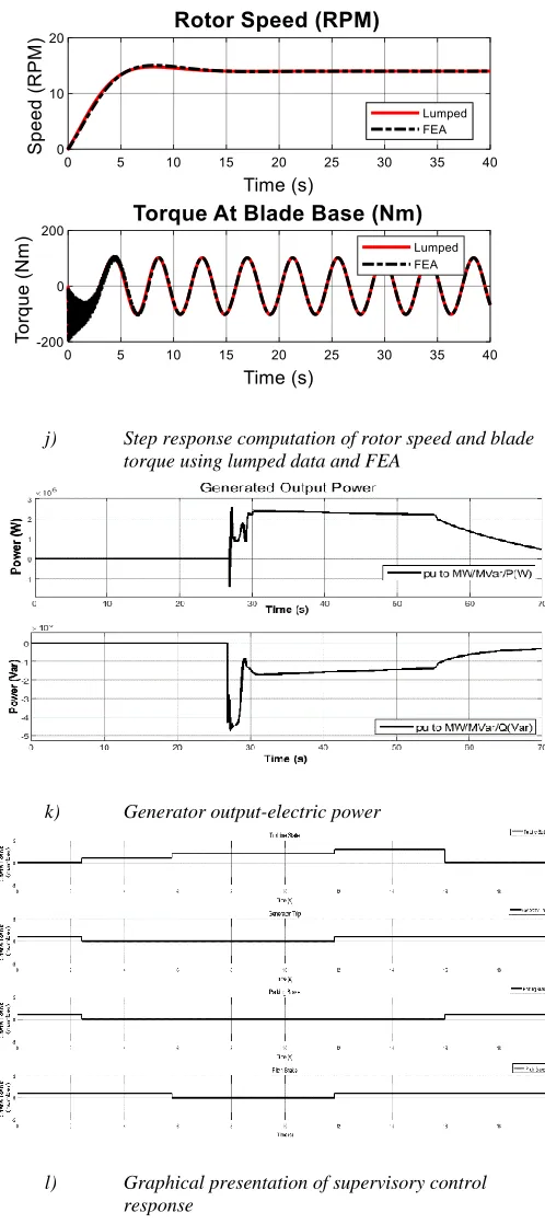
wind. To make the simulation more practical, we made variation in both wind speed and direction with time and chose the ‘varying wind’ block as input. Fig. 9b shows pitch control waveforms where the blue color indicates the input command and black color indicates the output which is following the pitch command. To find out the hydraulic actuator requirements, at first we have used ideal actuator in the pitch system. Fig. 9c shows the behavior of ideal actuator i.e. pitch angle variation with the input command and actuation force. The hydraulic actuator should be designed as per these results. Fig. 9d depicts the cylinder piston velocity for both ideal (black) and hydraulic (blue) actuators where the piston is linked with the blades. The performance is nonlinear in nature. A comparison between the performance of ideal and hydraulic actuator is shown in Fig. 9e. The hydraulic actuator force is quite acceptable as it remains almost similar with the ideal actuation force curve and finally we can keep the pitch control system with that performance in hand. Now we will focus on yaw control system and likewise pitch control we will use an ideal actuator to determine yaw torque requirement for our system. The torque curve for ideal actuator is shown in Fig. 9f. Fig. 9g indicates the nacelle’s yaw movement as per given yaw command and nacelle yaw rate (degree per sec) which is below 0.5 degrees complies with design requirements. Now with these two data sets, we can find out the required torque for servomotor actuation. Fig. 9h shows a comparison between two yaw actuators- ideal (red) and servomotor (black) actuator. The generated torque by using servomotor actuators are pretty good as following the nature of ideal actuator. Fig. 9l interprets the supervisory control system namely the states of the turbine- turbine startup, generator trip, parking and pitch brake which are pretty much convenient as per event-based control algorithm. Lastly, Fig. 9i shows our main control objective which is controlling the rotor speed with variousoperating conditions. It is evident from the curve that when time is zero, the rotor is at parking position. After sometime when wind strikes the blades it starts to turn slowly. When the wind speed exceeds the cut in speed after 30 seconds, the rotor has reached its maximum rotational speed which is approximately 15 rpm and remained steady up to next 30 seconds and goes to generating mode. After 70 seconds, the wind reached the cut-off speed, so the rotor needs to be stopped to avoid unnecessary damage and from the response curve, we can see, the rotor speed is gradually decreasing and finally reaches to zero i.e. in parking mode. From this region, maximum safe electrical power is given up to the cut-off speed, which is the speed of wind that is no longer safe to run the turbine [22]. Therefore, we can conclude that the supervisory control system is maintaining the desired linkage between pitch and yaw controllers, respectively. Fig. 9k shows the estimation of generated output power. As we can see, the rotor speed gets the steady value after 30 seconds and so as the power reaches its maximum value which is more than 2MW and keeps a steady state till 55 seconds, then decreases as the rotor speed slows down. Fig. 9j indicates the step response of two different iterative methods named as Lumped Parameter Model and
matrix based Finite Element Analysis (FEA) calculating the rotor speed and torque at the blade base and both results are identical. The rotor speed is showing steady with no overshoot, on the other hand torque curve is oscillatory in nature but bounded by the limiting values. Selecting an efficient control system requires doing tradeoff studies in early stages to determine which will provide enough force or torque while drawing the least power. The actuator must be developed together with the control systems and there may be multiple control loops that must interact with the actuation system.
a) Input wind speed and direction
c) Behavior of Ideal Actuator (Pitch system)
d) Cylinder piston velocity requirements for hydraulic actuator
e) Comparison between ideal and hydraulic actuator
performance (pitch control)
f) Torque requirement for Ideal Actuator
g) Yaw angle and rate of change of Nacelle
h) Comparison between ideal and servomotor actuation
performance (yaw system)
j) Step response computation of rotor speed and blade torque using lumped data and FEA
k) Generator output-electric power
l) Graphical presentation of supervisory control
[image:10.612.48.297.55.614.2]response
Figure 9: Simulation results for pitch, yaw and supervisory control systems
CONCLUSION
As the world is currently facing an energy and climate crisis, the development and utilization of alternative sources of energy has become an important challenge. Among the available renewable energy sources, wind energy proved to be one of the
cleanest and most reliable solutions for electrical energy production. The complexity of control systems in wind turbines is expanding rapidly and their design can be the difference between an immensely profitable system and a dormant or damaged system. Designing a robust control system requires an accurate model of the plant and tools that enable rapid iteration to find the best design. The control system must be optimized as possible while meeting multiple and sometimes conflicting system requirements. Pitch and yaw controllers must interact with supervisory logic controller in order to operate and protect the turbine under a wide range of environmental and statutory conditions. We have used linear control theory (Root locus, Bode plot, ITAE) to tune the controller parameters. After getting linearized model, we applied it to test the overall nonlinear model using Simulink design optimization. The simulation results show that the classical PI controller performs well, adjusts accurately the blade pitch angle so that the rotor turns at a sequential speed with the generator shaft and required yaw movement to change the nacelle position. To build this model in MATLAB, we have used Simscape multibody, Simmechanics, Simhydraulics, Control system toolbox and State machine [23]. It allows us the ability to simulate the physical systems such as mechanical, electrical, hydraulic and various control systems in a single environment. It enables engineers to incorporate requirements into the development process, design at the system level and to predict and optimize overall system performance without relying on only hardware prototypes as well as minimizing the cost.
FUTURE WORK RECOMMENDATIONS
APPENDIX
Part A
Results of Linearization of the Wind Turbine Equation
𝐾11= [𝐾𝑣𝑜𝑝
3
𝑅𝜔𝑡𝑜𝑝(0.44 − 0.0167𝛽𝑜𝑝) ∙
𝜋𝑅 𝑣𝑜𝑝(15 − 0.3𝛽𝑜𝑝)
∙ cos {𝜋 ( 𝜆𝑜𝑝− 3 15 − 0.3𝛽𝑜𝑝)}]
𝐾12= − 𝐾𝑣𝑜𝑝
3
𝑅𝜔𝑡𝑜𝑝2(0.44 − 0.0167𝛽𝑜𝑝) sin [𝜋 (
𝜆𝑜𝑝− 3 15 − 0.3𝛽𝑜𝑝)]
𝐾13= −0.00184 (𝛽𝑜𝑝𝑣𝑜𝑝2+
3𝛽𝑣𝑜𝑝3
𝑅𝜔𝑡𝑜𝑝2
) 𝐾
𝐾21=3𝐾𝑣𝑜𝑝
2
𝑅𝜔𝑡𝑜𝑝 (0.44 − 0.0167𝛽𝑜𝑝) sin [𝜋 (
𝜆𝑜𝑝− 3
15 − 0.3𝛽𝑜𝑝)]
𝐾22= −
𝐾𝑣𝑜𝑝3
𝑅𝜔𝑡𝑜𝑝(0.44 − 0.0167𝛽𝑜𝑝) ∙
𝜋𝜆𝑜𝑝 𝑣𝑜𝑝2(15 − 0.3𝛽
𝑜𝑝)
∙ cos {𝜋 ( 𝜆𝑜𝑝− 3 15 − 0.3𝛽𝑜𝑝)}
𝐾23= −0.00184𝐾 (2𝑣𝑜𝑝𝛽𝑜𝑝−9𝛽𝑜𝑝𝑣𝑜𝑝 𝜆𝑜𝑝 )
𝐾31= −
0.0167𝐾𝑣𝑜𝑝2
𝜆𝑜𝑝
sin [𝜋 ( 𝜆𝑜𝑝− 3 15 − 0.3𝛽𝑜𝑝
)]
𝐾32
=0.0167𝐾𝑣𝑜𝑝
2
𝜆𝑜𝑝 (0.44
− 0.0167𝛽𝑜𝑝) [0.3𝜋 ( 𝜆𝑜𝑝− 3
15 − 0.3𝛽𝑜𝑝)] cos {𝜋 (
𝜆𝑜𝑝− 3
15 − 0.3𝛽𝑜𝑝)}
𝐾33=
0.00184𝐾(𝜆𝑜𝑝− 3)𝑣𝑜𝑝2
𝜆𝑜𝑝
Part B
Wind Turbine Model and Simulation Parameters
1. Blade Requirements
Type
description AL 40
Blade length 40 m
Material Carbon/wood/glass/epoxy
Standard
color RAL 7035
Gloss Class 2: (30-70%) to be measured
acc. to DS/ISO2813
Type of rotor
air brake Full blade
Blade profiles FFA - W3, NACA 63.4
Twist 20°
Largest chord 3.08
2. Brakes Requirements
Mechanical
Type description Active Brake
Brake disc
Steel, mounted on high speed shaft
Number of calipers 2 piece
Brake Hydraulics
Voltage 3 x 480 V
Working pressure
range 140-150 bar
Oil capacity 11
3. Environment Requirements
Temperature interval for operation -30 to +30°C
Temperature interval for structure -40 to +50°C
4. Gear Train Requirements
Type description 1. step planet, 2. step helical
Gear house material Cast
Ratio 1:84.3
Mechanical power 1800 kW
Bending strength acc. to
ISO 6336 SF > 1.6
Surface durability acc. to
ISO 6336 SH > 1.25
Scuffing safety acc. to
Shaft seals Labyrinth
Oil sump App. 250 l
5. Generator Requirements
Type description 1 speed generator,
water cooled
Rated power 1650 kW
Apparent power 1808 kVA
Rated current IN 1740 A
Max power at Class F PFma 1815 kW
Max current at Class F
IFmax 1914 A
No load current I0 430 A
Reactive power
consumption at rated power (tolerance. acc to IEC 60034-1)
740 kvar
Reactive power consumption at no load (tolerance. acc to IEC 60034-1)
447 kvar
Number of poles P 6
Synchronous rotation speed
n0 1200 rpm
Rotation speed at rated
power nN 1214 rpm
Slip at rated power sN 0.0117
Voltage UN 3 x 600 V
Frequency F 60 Hz
Coupling Δ
Enclosure IP54
Insulation class/
Temperature increase F/B
6. Main Controller Requirements
7. Nacelle Requirements
Material EN-GJS-400-18U-LT EN-GJS-400-18U-LT
Standard colour RAL 7035 RAL 7035
Corrosion class, outside Acc. to DS EN ISO 12944:C5 I
Acc. to DS EN ISO 12944:C5 I
Rotor
Number of blades 3 pieces 3 pieces
Tip speed (synchronous) 61.8
m/s 61.8 m/s
Rotor shaft tilt 5° 5°
Eccentricity (tower center to
hub center) 3447 mm
Solidity (Total blade area/rotor
area) 0.05
Rotor orientation Upwind
8. Pitch Actuation Requirements
Hydraulic pressure 2e7 Pa
Annual average wind speed 8.5
m/s 8.5 m/s
Wind shear 0.20 0.2
Extreme wind speed 42.5 m/s (10 min.
average)
Survival wind speed 59.5 m/s (3
sec. average) 59.5 m/s (3 sec. average)
Automatic stop limit 20 m/s (10
min. average) 20 m/s (10 min. average)
Re-cut in 18 m/s (10 min.
average) 18 m/s (10 min. average)
Characteristic turbulence intensity
16% (including wind farm turbulence)
Accumulator Capacity 0.1 L
Accumulator Preload Pressure 1.5e7 Pa
Accumulator Maximum Pressure 2.5e7 Pa
9. Pitch Controller Requirements
Track angle within 1 degree
Rise Time 3 seconds
Settling Time 5 seconds
Proportional Gain, Kp 92845
Integral Gain, KI 307
10. Yaw Actuation Requirements
Type description Planetary gear
motor
Gear ratio of yaw gear unit app. 1:1687
Voltage 3 x 480 V
Rotational speed at full load 1140 rpm
Number of yaw gears 4 pieces
Yaw Brake Hydraulic disc
brake
Number of Yaw Friction
Units 6 pieces
Voltage 3 x 480 V
Working pressure range 140-150 bar
Oil capacity App. 10 l.
11. Yaw Controller Requirements
Max Yaw Rate 0.5 deg/sec
Rise time 3 seconds
Settling time 5 seconds
Proportional Gain, Kp 300
Integral Gain, KI 0.1
12. Tower Requirements
Type Description Conical,
tubular Conical, tubular
Material Welded steel plate Welded steel plate
Corrosion class, outside Acc. to DS EN ISO 12944: C5 I
Acc. to DS EN ISO 12944: C5 I
Colour RAL 7035 RAL 7035
Access conditions
Internal, safety harness, ladder
cage
Part C
3D Modeling Structures built in SimulinkTM
1. Overall Wind Turbine Model
3. Blade Mechanics Model
4. Nacelle Model
5. Pitch Mechanism Model
6. Hydraulic Actuator Model
7. Gear train Model
8. Generator Model
10. Servomotor Model
11. Tower Model
12. Grid Model
REFERENCES
[1] Kahrl F, Williams J, Jianhua D, Junfeng H. Challenges to China’s transition to a low carbon electricity system. [J] Energy Policy. 2011;39:4032-41.
[2] GWEC. Global wind report: Annual market update 2015. [M] GWEC,
Brussels; 2016.
[3] Wind Electricity Net Generation. International Energy Statistics. [M] EIA. Retrieved 2019-02-09.
[4] Wind Electricity Installed Capacity. International Energy Statistics. [M] EIA. Retrieved 2019-02-09. Source: Wikipedia
[5] Trevor M. Letcher, (2017), Wind Energy Engineering, A Handbook For onshore and offshore Wind Turbines, 125 London Wall, London EC2Y 5AS, UK. [B]
[6] Ackerman, (2000), Wind energy technology and current status: a review. Renewable and Sustainable Energy Reviews, [Online] 315-374. [B]
[7] Ackerman, (2005), Wind Power in Power Systems. Wiley, England. [B]
[8] Can Huang, Studies of Uncertainties in Smart Grid: Wind Power
Generation and Wide Area Communication. [T] Ph.D diss.,University of Tennessee, 2016
[9] Jacopo Antonelli, Reduced order modelling of wind turbines in MATLAB for grid integration and control studies, 1-20. [J]
[10] Balas, M. Fingersh, L. Johnson, K. Pao, L.(2006) Control of Variable-Speed Wind Turbines: standard and adaptive techniques for maximizing energy capture, [J] IEEE Control Systems Magazine, [Online] 26, 70-81.
[11] Boukhezzar, B. Siguerdidjane, H. (2005) Nonlinear Control of Variable Speed Wind Turbines without wind speed measurement. IEEE Conference on Decision and Control, [Online] 3456-3461.
[12] YE Hang-ye, ‘Control technology of Wind turbine generator’[M] China Machine Press, 2002.
[13] Simon De Zutter ; Jeroen D. M. De Kooning ; Arash E. Samani ; Jens
Baetens ; Lieven Vandevelde (2017) Modelling of Active Yaw Systems for Small
and Medium Wind Turbines, [P] IEEE 52nd International Universities Power
Engineering Conference (UPEC).
[14] Lubosny, Z. (2003) Wind Turbine Operation in Electric Power Systems.[P] Springer, Germany.
[15] Jasmin Martinez, Modelling and Control of Wind Turbines, [T] Master’s Thesis, Department of Process Systems Engineering, Imperial College of London, UK, 2007.
[16] H. M. Hassan, W. A. Farag, M. S. Saad, A. L. Elshafei, “Robust Dynamic Output Feedback Pitch Control for Flexible Wind Turbines” [P], IEEE EnergyTech 2012, May 29, Cleveland, Ohio, USA.
[18] Kari Medby Loland, Wind Turbine Yawed Operation, 1-59 [B]
[19] L. Wenzhou, C. Changqing, and Z. Zhuo, “Design of a large scalewind turbine generator set yaw system”, [P] IEEE Inter. Conf. on Computer Science and Education, Singapore, August 2011.
[20] W. Farag, M. El-Hosary, A. Kamel, K. El-Metwally, ( 2017) ‘A Comparative Study & Analysis of Different Yaw Control Strategies for Large Wind Turbines’[J] IEEE#41458-ACCS'017&PEIT'017, Alexandria, Egypt.
[21] Fernando G. Martins, (2005) ‘Tuning PID Controllers using the ITAE Criterion’, [J] Int. J. Engng Ed. Vol. 21, No. 5, pp. 867-873.
[22] A. Pintea, D. Popescu, P. Borne, ‘Modeling and Control of Wind Turbines’ LSS2010 (12th LSS symposium, Large Scale systems: Theory and Applications), Jul 2010, Lille, France. Hal-00512206. [P]
[23] S.Miller, webinar on Wind Turbine Model, Mathwork.Inc, March 2013.
Tang Wei: Doctoral tutor, Professor
of School of Electrical and Control Engineering, Shaanxi University of Science and Technology. The main research direction is paper disease detection, pulp and paper process automation, industrial process advanced control, large time delay process control and application. Tel: 13892980876; E-mail: [email protected]
Md. Muhie Menul Haque
(Correspondence Author): Post
graduate master’s degree student, School of Electrical and Control Engineering, Shaanxi University of Science and Technology. The main research diection is control theory and automation. He completed his bachelor of science in mechanical engineering from Bangladesh University of Engineering and Technology (BUET).
Tel: 15686068712; E-mail: [email protected] .
Shi Yong: Master’s instructor, Professor of School of Electrical and Control Engineering, Shaanxi University of Science and Technology. The main research direction isresearch on new power electronic circuit topology and its application, research on key technologies of reliability of power electronic systems. Tel: 13891884297; E-mail: [email protected]
Liu Yan: Doctoral student; Lecturer
of Shaanxi University of Science and Technology; Main research field: signal processing and virtual instrument. Tel: 13991892812; E-mail: [email protected]