Essays on Alternative Perspectives on Cross Border B2B Trust and Commitment

Georgia State University

ScholarWorks @ Georgia State University

Geosciences Theses Department of Geosciences

5-2-2018

SPATIOTEMPORAL VARIATION OF

LAND-USE AND LAND-COVER IN THE NAIROBI

RIVER WATERSHED, AND ITS EFFECTS ON

THE INORGANIC GEOCHEMISTRY OF

NAIROBI RIVER

Follow this and additional works at:https://scholarworks.gsu.edu/geosciences_theses

This Thesis is brought to you for free and open access by the Department of Geosciences at ScholarWorks @ Georgia State University. It has been accepted for inclusion in Geosciences Theses by an authorized administrator of ScholarWorks @ Georgia State University. For more information, please [email protected].

Recommended Citation

MUCHEMI, FRANCIS, "SPATIOTEMPORAL VARIATION OF LAND-USE AND LAND-COVER IN THE NAIROBI RIVER WATERSHED, AND ITS EFFECTS ON THE INORGANIC GEOCHEMISTRY OF NAIROBI RIVER." Thesis, Georgia State University, 2018.

RIVER WATERSHED, AND ITS EFFECTS ON THE INORGANIC GEOCHEMISTRY OF

NAIROBI RIVER

by

FRANCIS MUCHEMI

Under the Direction of Daniel M. Deocampo, PhD

ABSTRACT

Determining the effects of LULC and development on natural resources is necessary for

sustainability. This study focused on LULC changes in NRW over the past 3 decades and the

effects it had on the geochemistry of NR channel’s sediment. Impervious surfaces increased from

2.5% to 11.9%. Samples from the urban class had elevated levels of contaminants than other

classes. The concentrations of major inorganic elements were normal compared to the juvenile

UCC except MnO and P2O5 that were heterogeneously distributed and significantly enriched.

Heavy metals exhibited high DR than USEPA SSL in urban. Pb, Ce and Sb had the highest

concentration of 3400, 769 and 187.5 ppm respectively in the urban class. Heterogeneously

distributed and enriched elements like Pb, Y, Yb, Zr, Er,Ce, Zn, Lu, Sm, Th, Nd etc., were

attributed to humans’ input. Minerals identified were smectite, kaolinite, quartz, anorthoclase and

RIVER WATERSHED, AND ITS AFFECTS ON THE INORGANIC GEOCHEMISTRY OF

NAIROBI RIVER

by

FRANCIS MUCHEMI

A Thesis Submitted in Partial Fulfillment of the Requirements for the Degree of

Master of Science

in the College of Arts and Sciences

Georgia State University

Copyright by Francis Ndiritu Muchemi

RIVER WATERSHED, AND ITS AFFECTS ON THE INORGANIC GEOCHEMISTRY OF

NAIROBI RIVER

by

FRANCIS MUCHEMI

Committee Chair: Daniel Deocampo

Committee: Crawford Elliot

Lawrence Kiage

Electronic Version Approved:

Office of Graduate Studies

College of Arts and Sciences

Georgia State University

DEDICATION

I dedicate this thesis to my wife, Joyce and my two lovely daughters Shemmy and Stacy

ACKNOWLEDGEMENTS

To start with, I would like to express my heartfelt gratitude to my thesis advisor Prof.

Daniel Deocampo for the immense support he accorded me to be able to complete this thesis

research. I relied on his guidance, motivation, patience, and knowledge at all times to write this

thesis. Dr. Deocampo also offered me a graduate research assistant opportunity that allowed me to

sail through my four semesters on Campus with a lot of ease. I would not have envisaged having

a better mentor and advisor for my M. Sc. studies.

Besides my advisor, I sincerely thank the rest of my thesis committee; Prof. Lawrence

Kiage and Prof. Crawford Elliott for their dedicated and insightful contributions and moral support.

I also want to thank Prof. Dajun Dai for the excellent assistance in watershed delineation and

analysis work. My sincere gratitude goes to the Department of Geosciences, Georgia States

University for offering me a graduate teaching assistance opportunity that also facilitated my four

semesters on Campus.

I appreciate and acknowledge the opportunity given to me by the National Museums of

Kenya for allowing me to be out to study on a two years’ study leave.

I also want to thank my fellow course mates who contributed in one way or the other to the

completion of this thesis. Many thanks to my office mate Benjamin Opiyo for being a ‘brother’

during all that time, Nathan Rabideaux, David Davis, Lanier Henson, Vicky Cheruiyot, Alireza

TABLE OF CONTENTS

ACKNOWLEDGEMENTS ... V

LIST OF TABLES ... IX

LIST OF FIGURES ... X

LIST OF ABBREVIATIONS ... XII

1 INTRODUCTION ... 1

1.1 Literature Review ... 1

1.1.1 Land-use and Land-cover ... 1

1.1.2 Geochemistry ... 3

1.1.3 The Nairobi River Watershed ... 6

1.2 Goal and Objectives ... 8

1.3 Hypotheses ... 8

1.4 Justification of the Study ... 9

2 METHODS ... 10

2.1 Study Area ... 10

2.1.1 Water Resources ... 10

2.1.2 Geology of Nairobi River Watershed, Kenya ... 14

2.1.3 Soil ... 15

2.1.4 Climate ... 17

2.3 Geochemistry ... 19

2.4 Mineralogy ... 21

2.5 Loss-on-ignition Analysis ... 23

2.6 Statistical Analysis and Data presentation ... 24

3 RESULTS ... 24

3.1 Nairobi River Watershed Delineation ... 24

3.2 Land-Use and Land-cover ... 25

3.2.1 Multispectral Landsat Images ... 25

3.2.2 LULC Change Detection ... 27

3.3 Geochemistry ... 32

3.3.1 Major Elements ... 32

3.3.2 Trace Elements ... 35

3.3.3 Upper Continental Standardized Spider Diagrams ... 40

3.3.4 Chemical index of alteration (CIA) and loss on ignition ... 43

3.4 Mineralogy ... 48

3.4.1 Bulk Minerals ... 48

3.4.2 Clay Minerals ... 50

3.5 Loss-on-Ignition ... 54

4 DISCUSSION ... 54

REFERENCES ... 61

Appendix A Inorganic Element Data ... 68

Appendix A.1 Major oxides ... 68

Appendix A.2 Major Oxides, LOI, Total, Carbon and Sulfur ... 69

Appendix A.3 Geochemical Analysis ... 70

Appendix A.4 Geochemical Analysis ... 71

Appendix A.5 Geochemical Analysis ... 72

Appendix A.6 Geochemical Analysis ... 73

LIST OF TABLES

Table 1 LULC classification of Nairobi River Watershed in 1986 and 2015 ... 28

Table 2 LULC gains and loses between 1986 and 2015 ... 32

Table 3 Distribution of major elements down Nairobi River gradient ... 33

Table 4 Concentration of heavy metals in ppm ... 35

Table 5 Concentration of primary heavy metals in ppm... 38

Table 6 Comparison of percent weight of main elements, CIA, LOI and Rb in ppm ... 43

Table 7 Bulk mineral composition ... 48

Table 8 Clay mineral composition ... 52

LIST OF FIGURES

Figure 1 Nairobi City political boundaries and Rivers ... 11

Figure 2 Ondiri Swamp ... 12

Figure 3 Solid waste along Nairobi River... 13

Figure 4 Geology of Nairobi River Watershed ... 14

Figure 5 Soil survey map ... 16

Figure 6 Köppen-Geiger Climate Type ... 17

Figure 7 Total annual rainfall and average temperature from 1985 to 2015 ... 18

Figure 8 Nairobi River Watershed ... 25

Figure 9 Multispectral Landsat images used in the study ... 25

Figure 10 subsets of Landsat images showing the area of interest in false color ... 26

Figure 11 LULC change image ... 27

Figure 12 LULC of Nairobi River Watershed in 1986 and 2015 ... 28

Figure 13 LULC Change, Urbanization and Deforestation ... 29

Figure 14 LULC Change, Agriculture and Deforestation ... 31

Figure 15 LULC gains and losses between 1986 and 2015 ... 32

Figure 16 Distribution of major elements down the river gradient ... 34

Figure 17 Distribution of major elements without SiO2 ... 34

Figure 18 Distribution of heavy metals ... 36

Figure 19 LULC and samples collection points ... 37

Figure 20 Concentration of trace elements down the river gradient ... 39

Figure 21 Comparison of concentration of heavy metals to allowable limits ... 40

Figure 22 Enrichment/depletion of selected elements against the UCC values ... 41

Figure 24 Comparison of CIA, LREE/HREE and La/Yb ratios ... 45

Figure 25 The general trend of REE along the river gradient ... 46

Figure 26 General trend of Sample elements/UCC down river gradient ... 47

Figure 27 XRD peaks for combined bulk mineralogy ... 49

Figure 28 XRD peaks for combined clay mineralogy ... 50

Figure 29 A graph showing air dried, glycolated and heated clay peaks ... 51

Figure 30 Air dried and formamide treated clay peaks ... 53

Figure 31 Loss-on-ignition ... 54

LIST OF ABBREVIATIONS

CIA – Chemical Index of Alteration DEM – Digital Elevation Model DR – Detection Ratio

GIS – Geographic Information System HREE – Heavy Rare Earth Elements

ICP-AES – Inductively Coupled Plasma Atomic Emission Spectroscopy ICP-MS - Inductively Coupled Plasma Mass Spectrometry

LOI – Loss on Ignition

LREE – Light Rare Earth Elements LTV – Long-term Trigger Value LULC – Land-use and Land-cover Ma – Million years ago

MR – Mathare River NR – Nairobi River

NRBP – Nairobi River Basin Rehabilitation Program NRW – Nairobi River Watershed

OLI – Operational Land Imager PPM – Parts Per Million

REE – Rare Earth Elements RS - Remote Sensing

SSL – Soil Screening Levels STV – Short-term Trigger Value TM – Thematic Imager

UCC - Upper Continental Crust

USEPA – United State Environmental Protection Agency USGS – United States Geological Survey

1 INTRODUCTION

1.1 Literature Review

Human population growth in urban environments, economic development, and demand for

growing need for food, water, and other basic needs has grown considerably. As a result, surface

and ground water have suffered immensely from pollution and excessive withdrawals emanating

from urban and agricultural areas (Shabnam et al., 2017). Both ground and surface water resources

are contaminated by pollutants associated with humans and animal fecal wastes, industrial

chemicals and other anthropogenic activities. Pathogenic microorganisms breed in these waters

and can cause risks to human health and water impairment especially in the tropics where

conditions favor the growth of microorganisms (Savichtcheva and Okabe, 2006; Tallon et al.,

2005).

1.1.1 Land-use and Land-cover

Understanding the effects of land-use and land-cover (LULC) on the quality of water in a

watershed, as well as detecting spatiotemporal changes of LULC is important for watershed

management. Information on LULC in a watershed and its dynamics is essential in providing bases

upon which decisions concerning watershed management can be anchored (Alphan, 2003).

Urbanization results in building of infrastructure like roads and industries that is meant to support

social-economical activities and thus increases the development of impervious surfaces on the

landscape (United Nations, 2017). These impermeable surfaces affect the quality of water, public

health, habitats, aquatic ecosystems, and reduce esthetic value of water in a watershed by altering

runoff (Uygun and Aldek, 2015; Schueler, 1994)). Runoff from urban areas and agricultural lands

may cause severe effects on downstream environment by contributing non-point source pollution.

This has become a priority in monitoring, prevention, and restoration of surface water quality in

the flow of polluted runoff into the waterbodies through a network of channels and pipes (Arnold

and Gibbons,1996). Remote Sensing (RS) is a technology utilized to determine spatiotemporal

LULC (Foody, 2002), while Geographic Information System (GIS) is a flexible tool for collection,

storage, display and analysis of digital data required for landscapes’ classification and change

detection (Demers, 2005). The popularity of RS and GIS technologies have led to an increase in

studies focusing on quality and pollution of water, including mapping, modeling pollution sources,

drinking water quality and assessing water pollution levels (Coskun et al., 2008; Foster et al.,

2000).

Human/nature interaction has resulted in deforestation, increased sedimentation, reduction

in net primary productivity and reduced soil quality all on a backdrop of climate change (Dwivedi

et al., 2005). To better understand these processes, remote sensing images from satellite can be

used to classify LULC properties in a watershed. Land-use in remote sensing is different from

land-cover, and is defined as activities applied by humans on the land (Cihlar and Jansen, 2001).

Mixing of land-cover and land-use in remote sensing is common for environmental assessments

(Jansen and Di Gregorio, 2002). Multi-temporal and multispectral satellite images are analyzed

and converted into spatiotemporal information, vital for understanding and evaluating

development processes and patterns for developing LULC datasets (Steininger, 1996). Different

classification methods are used in which pixels are grouped into related spectral classes by

clustering algorithms. ERDAS-ERDAS imagine is a remote sensing image processing software

that uses both supervised and unsupervised classification systems to classify digital images, with

the later applying iterative self-organizing data analysis technique (ISODATA). ISODATA

clusters pixels using iteration whereby, it recalculates the average and cluster pixels according to

classification in which pixels with maximum likelihood are grouped into corresponding classes.

However, there is often misclassification and inaccuracy of digital images when using automatic

classification, especially when dealing with arid and heterogeneous landscapes. This inaccuracy is

caused by inter-annual variability of climate, resulting to a variety of spatial patterns, variable

vegetation cover, and high fragmentation (Barkhordari and Viardanian, 2012).

1.1.2 Geochemistry

Diffuse urban effluent via storm water and uncontrolled discharge of wastewater are the

primary causes of surface water contamination (Defra, 2012). Clays and soils can sorb cations of

many elements and compounds because most of them have surface charge. The presence of heavy

metals therefore in the bottom sediments of a river reveal a history of pollution either from a human

source or natural origin. This study determined the concentrations of major elements of the Earth’s

crust from Nairobi River, heavy metals of concern and other trace elements. Heavy metals occur

naturally at a low level but may escalate to high concentrations because of anthropogenic activities

such as sewage, irrigation, mining and smelting (Niu et al., 2013). Potassium (K) and

Orthophosphate (PO4) ratios, ammonia concentration above 0.3 mg/L and boron (B) ion

concentration above 1.0mg/L are indicators of gray water in surface water bodies (Panasiuk et al.,

2015). Heavy metals are usually considered ecologically toxic, persistent and bioavailable

contaminants because they are health hazards to animals, trees and the ecosystems (Zhang et al.,

2015).

The presence of arsenic (As) in surface water may be contributed by groundwater sources

linked to geological sources. Arsenic is responsible for hyperkeratosis and vascular diseases in

humans. Arsenic gets into the air from volcanic activities, wind erosion, volatilization from soil,

1989). About 18,800 tons of As per year which is about 30% of the global total As into the

atmosphere is as a result of human activities (Nriagu and Pacyna, 1988). Cadmium is spread into

the air by anthropogenic activities of mining and smelting, as well as usage of phosphate fertilizers,

sewage, and other industrial usages like manufacturing of batteries, pigments, plating, plastics, etc.

(ATSDR, 1999). Cadmium (Cd) causes kidney problem, a dysfunction caused by a reduction of

glomerular filtrate. Lead (Pb) causes mental disorders in children who may develop problems with

memory, learning, and concentration. Pb may also cause anemia because it inhibits the formation

of hemoglobin. Chronic exposure to mercury even in small quantities in drinking water may cause

psychological and neurological symptoms like tremor, restlessness, anxiety, stress, and depression.

Antimony is emitted into the environment mostly as a result of coal burning or with fly ash during

the melting of antimony-containing ore (Nriagu & Pacyna, 1988). Oral exposure to high levels of

antimony(III) has been associated with optic nerves destruction, retinal breeding, uveitides and

could trigger premature birth (Stemmer, 1976). Presence and quantity of these metals were

determined in the Nairobi River because even though people may not be drinking water from the

river, the water is used mainly for small-scale irrigation projects and the produce is sold to

unsuspecting city residents. There are three primary pathways through which humans are exposed

to heavy metals: direct ingestion, inhalation, and through skin contact. Ingestion and skin contact

exposures are prevalent for elements that are dissolved in water. Children are at a higher risk from

exposure to heavy metals than adults because they have a higher rate of cell division (Saha et al.,

2016). A study done along the Nile delta showed a disproportionate distribution of heavy metals,

i.e., As, Pb, Cd, and Hg with respect to season, geographical area and sampling points in the Nile

Delta, Egypt (El-Kowrany et al., 2016). The severe intensity of all these metals is present in all

the concentration of most metals with increasing distance from the point of introduction. However,

some elements have constant values even over great distances, for instance As and Mn (Saha et

al., 2016). This has been explained as a result of natural sources rather than anthropogenic

introduction (Saha et al., 2016). The general considered range of carcinogenic risks for As when

ingested or in contact with the human skin is10-6 to 10-4 mg/Kg (ppm) by USEPA (2012) standards.

Freshwater contamination by trace metals in the developing countries has become a major

environmental concern (Goher et al., 2014a). Anthropogenic inputs of pollution are rapid and

intense, as opposed to natural contamination which is gradual and slow through weathering and

leaching (El-Bouraie et al., 2010). Many trace elements above normal are produced by industries,

domestic wastes, storm-water from urban areas, landfills and agricultural chemicals (Hashim et

al., 2011). Most inorganic pollutants are of significant environmental concern because they are

usually non-biodegradable, have a long biological half-life and toxic to plants and animals (Goher

et al., 2014b; Singare et al., 2012). Some trace metal contaminants are very toxic even in small

concentrations and could lead to bio-accumulation when absorbed over a long time causing

damages to the nervous system and other internal organs like the liver and kidneys (Lohani et al.,

2008). Different countries have set long-term trigger values (LTV) and short-term trigger values

(STV) for heavy metals in irrigation water. These values refer to the maximum and minimum

acceptable contamination of water used to irrigate human food (Anzecc, 2000). World Health

Organization (WHO, 2006) and USEPA (2012) developed standards for acceptable limits for

heavy metals in water used for humans’ consumption.

The chemical index of alteration (CIA) is a calculation based on geochemical analysis that

has been applied for decades to study the history of silicate minerals weathering into clays (Roddaz

(Potter P.E. et al., 2005). It is a quantitative indicator for determining silicate weathering and is

defined as Al2O3/(Al2O3+CaO*+Na2O+K2O) x100%. CaO* is the amount of CaO in silicate

fraction and does not include CaO combined with phosphates and carbonates minerals, such as

may occur in soil carbonates or biogenic material (e.g. gastropod shells). To avoid potential

complications caused by pedogenic and biogenic carbonates, if CaO content is less than that of

Na2O, then the value of CaO is used in computing CIA. If the content of CaO is higher than that

of Na2O, then the value of Na2O is used in the equation instead of that of CaO. CIA reflects the

degree of aluminum silicate minerals, especially feldspar weathering into clay minerals (Fedo et

al., 1995). Higher CIA values indicate more chemical weathering and leaching of Na, K and Ca

bound minerals (Nesbitt, 1989). The degree of weathering is correlated to the denudation rate of

the watershed (Li et al., 2010). Li et al. (2010) further established that the degree of weathering is

also affected by average annual temperatures, latitude and the thickness of the soils layer.

Weathering activities are also affected by climate and runoff in latitudinal catchments while the

underlying bedrock and other factors are secondary (Shao J.Q, et al., 2012, Yang S.Y., et al. 2004).

River broadening and floodplains may cause enhanced values of CIA because of weathering of

floodplain sediments (Heller P.L. et al., 2001).

1.1.3 The Nairobi River Watershed

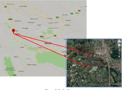
The Nairobi River flows through Nairobi City, the capital of Kenya (Figure 1) and is an important

resource in the watershed. The river originates from the Ondiri Swamp catchment (Figure 2), about

10 miles to the Northwest. The effect of urbanization is evident from a gradual change of the

physical appearance of the flowing water down the gradient and through the city. It is joined by

merges with the Athi River to the south of Nairobi and flow through the Eastern Province of Kenya

and into the Indian Ocean.

Most of the piped water (94%) consumed in Nairobi comes from the Aberdare Ranges to the

North of the city while the remaining 6% comes from Kikuyu spring and Ruiru Dam. Nairobi City

residents who do not have piped water rely on water vendors who charge them expensively for

water, unlike those privileged to have piped water from the County Government. It is estimated

that only 10% to 48% of the city residents are connected to the sewage line (Athi Water Services

Board, 2011). Two water treatment plants treat industrial and domestic wastes with a capacity of

112,000m3_{/day. One of the plants contains stabilization units with the most intensive pond systems}

in Africa, but only half the capacity has been in use (EACF, 2008). The effluent from these plants

is drained into the Nairobi River (NCWSC, 2011). Different groups and institutions have tried to

remediate the pollution of Nairobi River in the past, and one important body is Nairobi River Basin

Rehabilitation Program (NRBP). NRBP was created to bring together the government of Kenya,

development partners, private sector and civil societies to spearhead the management of the rivers

in the basin (African Development Bank, 2010). They determined the sources of pollution into the

rivers as coming from uncollected garbage, human wastes from informal settlements, industrial

wastes in the form of gaseous emissions, liquid effluents, agrochemicals, petrochemicals, metals

and overflowing sewers. A ten-points strategic plan was proposed to curb the proliferation of

pollution and they include stoppage of illegal discharge and development and implementation of

the integrated solid waste management system. Moreover, the benefits of rehabilitating and

maintaining the rivers’ system were enumerated, and they included provision of safe and clean

water, ecosystem services, economic improvement, employment, recreational, tourism, security,

Resources, Kenya, 2009). However, garbage and other human effluent along the banks of the

rivers’ channels are still a problem, and the water quality is still unpleasant by physical appearance.

1.2 Goal and Objectives

The main goal of this study was to compare the relationship between LULC within Nairobi River

Watershed with the quality of water in Nairobi River.

Objectives

i. To establish the extent of LULC change in the watershed for the past three decades

(between May 1986 and May 2015).

ii. To determine the rate of urbanization leading to the creation of impervious surfaces in

the watershed

iii. To delineate the Nairobi River watershed and determine the current proportions of

LULC.

iv. To determine the concentrations of inorganic elements and mineralogy of the Nairobi

River channel’s sediments.

v. To establish the relationship between the concentrations of inorganic elements, LULC,

and the distance from the origin of Nairobi River.

1.3 Hypotheses

i. There has been a significant change of LULC in Nairobi River Watershed in the past

3 decades.

ii. Development of impervious surfaces (urbanization) in the watershed have increased

iii. There is a significant amount of inorganic pollutants in Nairobi River as a result of

anthropogenic activities in the watershed.

iv. The amount of inorganic pollutants increased down the river gradient and it is

expected that the urban areas experienced more pollution than other classes.

1.4 Justification of the Study

There is a growing need for the provision of clean water to cater for the demands of the

ever-increasing humans’ consumption, irrigation and other uses in many parts of the world. These

requirements have been increased by contamination of existing water resources in crowded places.

The problem is expected to worsen in future because of the projected climate change that is likely

to affect the hydrological cycle, while at the same time the population is predicted to increase

rapidly especially in cities. It is logical for water managers to take stock and protect all the possible

sources of water especially the natural ones. One way of doing this is by trying to remediate the

polluted surface water by putting in place measures that will alleviate the menace of water

pollution and prevent future surface and groundwater contamination. To achieve this, toxicological

analyses of hydrological resources is necessary. Determination of the types and intensity of

contaminants in water assets, the establishment of possible sources of pollution and proposals for

practical ways in which rivers can be managed from pollution is paramount. This study determined

the type and sources of primary inorganic pollutants of concern in Nairobi River, an important

river flowing within the heart of Nairobi, the capital city of Kenya. It also sets a base upon which

city planners and water managers in Nairobi could apply measures that will address pollution

concerns in Nairobi Rivers. Moreover, there is hardly any published study that has been

2 METHODS

2.1 Study Area

2.1.1 Water Resources

The study was conducted in the Nairobi River, the main river flowing through Nairobi

City, Kenya. The River originates from Ondiri Swamp located about 10 miles northwest of the

city, and the swamp has an area of about 32ha. It is joined by other rivers and tributaries at different

points within the city before merging with the bigger Athi River to the south of Nairobi. Other

rivers and tributaries join the Nairobi River down the gradient, i.e., the Ruiru, Kamiti, Kasarani,

Ruaka, Karura, Gitathuru, Kirichwa, Motoine-Ngong, and Mathare Rivers. The rivers draining

the watershed are perennial, and there is a good aquifer between the Kerichwa Tuffs and the

underlying Nairobi phonolite (Figure 1 and 4). However, the fluoride content of the aquifer tends

to be high (Saggerson, 1991). Nairobi City got its name from the Nairobi River which is a Maasai

(a tribe in Kenya and Tanzania) translation for cool water. The City is located at 1°09′S 36°39′E

and 1°27′S 37°06′E, while its administrative boundaries encompasses a total area of 696 Km2 (269

Figure 1 Nairobi City political boundaries and Rivers

Figure 2 Ondiri Swamp

These are extracts from Google map showing the location of Ondiri Swamp, the origin of the main channel of

Nairobi River (Google Earth)

The rivers’ and tributaries’ within the city have been significantly encroached and abused,

with massive amount of solid wastes along the banks (Figure 3). Industrial wastes and domestic

sewage disposals are a big problem. In September 2016, the County government of Nairobi

mapped 278 polluters mainly factories in Nairobi industrial area. During the same time, there was

a mop-up campaign against residential houses that were not connected to the main sewage system

and several property owners that were found draining untreated wastes into the river were

apprehended (Daily Nation, Kenya, 2016). Those washing vehicles along the rivers were ordered

to acquire water recycling machines that could separate soaps and mud from water or otherwise

towards cleaning Nairobi River, but a lot more is required if the quality of water in the river is

expected to improve for safe human consumption.

Figure 3 Solid waste along Nairobi River

These are images captured along Nairobi River channel in the urban class and they show the extent

of solid waste contamination along the river. Plastic bags are a menace all along the river especially

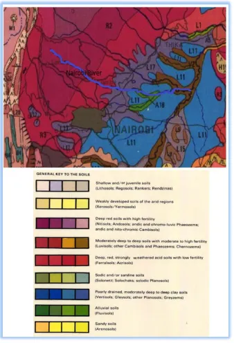
2.1.2 Geology of Nairobi River Watershed, Kenya

Figure 4 Geology of Nairobi River Watershed

The volcanic materials dominating the watershed are mainly phonolite, trachyte, and tuff

dating to Pliocene. The Northern and the Western regions are predominantly occupied by

Kerichwa tuff (Pka), Nairobi trachyte (Pnt) and Kinangop tuff (P-Kta-5) (Figure 4). The southern

part is mostly occupied by Nairobi phonolite (Pnp). Kerichwa and Kinangop tuffs date to about

3.34 to 3.70 ma., they are trachytic tuffs and are often welded and overlie the Nairobi trachyte

(Baker et al., 1988). There is a likelihood of bleaching and clay alterations which most likely

represents the weathering situation before the eruption of Limuru trachytes. Nairobi trachyte dates

to about 3.17 to 3.45 ma., and it is greenish and sometimes has tabular feldspar phenocrysts.

Nairobi Phonolite is the oldest of the Pliocene series, dating 5.20 ma. It is a black to blue material

that erupted as a number of flows. Lava is vesicular in the upper flow section but rarely contain

amygdule. These phonolites are easily distinguished from the Kapiti Phonolite because they lack

substantial phenocrysts (Saggerson, 1991).

2.1.3 Soil

The Nairobi River originates in an area with a deep red soil with high fertility, probably

nitisol and andosol soils (Figure 5). The city lies within a well-drained reddish soil in the north to

poorly drained, dark and moderately deep to deep vertisol to the south (Sombroek and Pauw van

der, 1980). Vertisols are soils with high proportions of expansive clay known as montmorillonite

that forms deep cracks under dry conditions. Vertisols have a deep A horizon but no B horizon

(Donovan, 1981). Nitisols are deep red soils with clay content of more than 30% and are found in

the tropics and subtropics. Nitisol support tropical rain forests and savannah vegetation but are

Figure 5 Soil survey map

A soil survey map and legend of Nairobi area (Adopted from Sombroek and Pauw van der, 1980). Nairobi

River originates from a more reddish and well drained soils in the northwestern side of NRW to a poorly

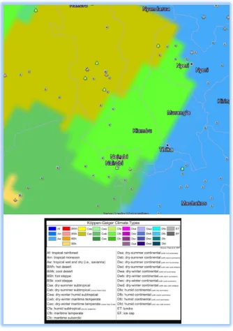
2.1.4 Climate

The Climate type of NRW is largely humid Sub-tropical but in the western side there is a significant portion

The data was retrieved from the World Bank Group, Climate Change Knowledge Portal for Development Practitioners and Policy Makers

The larger part of Nairobi area has a humid sub-tropical climate (Cfa) type according to

Köppen-Geiger Climate characterization. The western region of the watershed is dominated by the

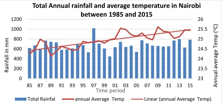
tropical wet and dry (Savanah) climate (Figure 6). The average annual precipitation remained very

constant in the last three decades except in the year 1997 when the total annual rainfall (1018 mm)

was higher because of El Niño -Southern Oscillation (ENSO) phenomenon (Figure 7). The lowest

annual precipitation of 448 mm was recorded in the year 2000 because of a prolonged drought.

The average annual temperature has, however, increased by about 1o_{C during this period, i.e., from}

24.5oC to 25.5oC.

2.2 Land-Use and Land-cover

Remote sensing and Geographic information system techniques were used to delineate the

Nairobi River Watershed and to classify LULC pattern. Multispectral Landsat digital images were

acquired from the United State Geological Survey (USGS) visualization viewer, GLOVIS

(http://glovis.usgs.gov) website and analyzed using ERDAS-ERDAS IMAGINE and ArcGIS

23 23.5 24 24.5 25 25.5 26 0 200 400 600 800 1000 1200

85 87 89 91 93 95 97 99 01 03 05 07 09 11 13 15 An

n u al av era ge T em p ( oC) Rain fall in mm Time period

Total Annual rainfall and average temperature in Nairobi between 1985 and 2015

Total Rainfal annual Average Temp Linear (annual Average Temp)

software for RS and GIS respectively. Both images were captured from Landsat satellites, one

from May, 1st 1986 and the other one from May, 1st _{2015. The 1986 image is a Landsat 5 TM}

(Thematic Mapper) while the 2015 image is a Landsat 8 OLI (Operational Land Imager), both

with a spatial resolution of 30 m for the main bands. Image rectification and atmospheric

corrections were performed on both images to improve the accuracy of the results. Delineation of

the watershed’s boundary was done using ArcGIS on a SRTM (Shuttle Radar Topography

Mission) digital elevation model (DEM) data of 90m resolution, obtained from USGS. Watershed

delineation processes from ArcGIS involved the filling of sinks in the DEM, flow direction and

accumulation, streams’ network and links and finally the area-wide drainage basin from a pour

point. All the stream orders draining water to Nairobi River were included in the watershed. The

watershed boundary layer was used to extract the study area from the Landsat images and then

used for further analysis. The two image extracts were classified using the unsupervised

classification method in ERDAS Imagine, whereby 20 iterations were set to determine 36 spectral

classes. From these spectral classes, five informational classes, i.e., water, forest, agriculture,

bare-ground, and urban were established, and the results from both images compared to detect the

change in LULC in the watershed from 1986 to 2015.

2.3 Geochemistry

The geochemistry of Nairobi River was based on sediment samples collected along the

river channel. Eight samples were selected randomly along the river and georeferenced. Two

samples (NR7 and NR6) were obtained from a more agricultural section of the watershed and less

developed. Four samples (NR5, NR4, NR3, and MR1) were collected from an increasingly

developed section. Sample MR1 was not picked from Nairobi River but from Mathare River, a

sample MR1 was picked near sample NR3 because they both represent the urban class in this

analysis. Sample NR2 was collected from a less developed part of Nairobi where urbanization is

currently spreading to. The last sample (NR1) came from adjacent the biggest sewage treatment

plant in Kenya and East Africa. This sample was meant to test the effects of the return flow from

the sewer treatment plant.

Analysis of inorganic elements was conducted on each sample, provided by the commercial

analytical company ALS Global (Reno, Nevada). Oxides of major elements were analyzed using

inductively coupled plasma (ICP) method coupled with Atomic emission spectrometry (AES). In

this analysis, samples were decomposed using lithium metaborate (LiBO2) or lithium tetraborate

(Li2B4O2) fusion. The concentration was calculated from the determined elemental concentration.

The compounds analyzed using this method were oxides of aluminum (Al2O3), barium (BaO),

calcium (CaO), chromium (Cr2O3), iron (Fe2O3), and magnesium (MgO). Others included

manganese (MnO), phosphorous (P2O5), potassium (K2O), silicon (SiO4), sodium (Na2O),

strontium (SrO), and titanium (TiO2). Inorganic sulfur and carbon were analyzed using LECO

technology which is a combustive technique for analyzing metals and alloys for sulfur, carbon and

some other elements. LECO analysis detects levels as low as 0.01% of both sulfur and carbon in a

sample. Base metals were analyzed using MS82 which is a four acid digestion technique for

analyzing ultra-trace levels. In this method, samples are decomposed using Lithium Metaborate

fusion and analyzed by Inductively Coupled Plasma – Mass Spectroscopy (ICP-MS). Volatile trace

elements were digested using aqua regia digestion and analyzed using ICP-MS. Major elements

2.4 Mineralogy

Each sample was analyzed at Georgia State University using Pert PRO PANalytical

X-Ray diffractometer equipment running from 0.5o to 45o for clay (oriented slides’) samples and 65o

for powdered samples, and the generator set at 45kV tension and 40mA current. This analysis was

to determine the mineral composition of the sediments. Determination of mineral composition was

vital because it explained whether the geochemistry of the channel sediments was as a result of

mineral precipitation or from anthropogenic activities. Soil fractions were separated using particles

settlement technique adopted from Jackson et al. (1950). This technique allowed sorting out of

four sediments fractions which included sand (> 50 microns), coarse silt (20 – 50 microns), fine

silt (2 -20 microns) and clay (< 2 microns). The procedure involved suspending the sediment in

distilled water and waiting for a specific duration of time before decanting. 2% sodium chloride

solution was added to bring the solution to a weaker base (about pH 9.5) to facilitate flocculation.

For larger particles of sand (>50 microns) settlement was timed for 40 seconds for every 4 inches

(10 cm) column height of the suspension, after all the particles had been suspended. The

supernatants were re-suspended, allowed to settle for 40 seconds per 4 inches’ column height of

the suspension and then decanted. Re-suspension and decanting were repeated several times until

all the clay and silt were separated from the sand. The >50 microns fractions were then dried at

50oC and ground to a finer powder for bulk minerals analysis with XRD.

After all the sand was extracted, the suspension was then stirred thoroughly for about 30

seconds until all the particles were well mixed in the suspension. Silt settlement was timed at 5

minutes for every 4 inches’ column height of suspension. After five minutes, the suspension was

carefully decanted, and the supernatant re-suspended in distilled water for 5 minutes for every 4

times until all the clays were removed, which was marked by attaining similar results after

consecutive cycles. This process removed all the particles within the range of 20 – 50 microns,

which were then dried at 50oC and ground into a fine powder. The larger grains (2-20 microns) in

the suspension were removed by letting the suspension settle for eight hours of every 4 inches

column height of the mixture, after which it was decanted. Petrographic Microscope slides were

prepared with the 2-20 microns supernatant and the rest dried at 50oC and then ground to a fine

powder for bulk minerals analysis with XRD.

Separation of < 2 microns fraction with the rest of the suspension was done by adding a

few drops of calcium carbonate solution to the mixture. Calcium carbonate hastens flocculation,

whereby all the particles settle after a couple of minutes, leaving behind a clear liquid. The clear

liquid was carefully decanted and the sediments re-suspended in distilled water and centrifuged

for eight minutes at 1100 rpm. The clear liquid was decanted and the samples suspended again in

distilled water and centrifuged. This process was repeated for a couple of times to wash the samples

off the calcium carbonate. Caution was, however, exercised to avoid resuspension of clay particles

into the distilled water when all the calcium carbonate was rinsed from the sediment. The

supernatants were used to prepared glass slides for clay minerals’ analysis using the X-Ray

Diffractometer. Two slides were prepared from each sample whereby each slide was done by

adding about 20cc of well-mixed clay and distilled water. The rest of the clay sediments were left

in the suspension. Mineralogy studies were conducted on powdered samples, i.e., sand (>50

microns), silt (20-50 microns) and finer particles (2-20 microns); and slides, i.e., clay (<2 microns).

The powdered fractions were analyzed for bulk analysis using PW 3064 sample stage

which is the most convenient for powdered samples. Clay samples on petrographic microscope

Four XRD patterns were conducted on clay samples to determine the clay mineralogy of Nairobi

River channel’s sediments. The following treatments were performed to determine the clay

mineralogy of NR.

1. Samples were air dried for about 24 hours before analysis with the XRD.

2. The air-dried samples were heated at about 550oC for one hour before the analysis

with the XRD.

3. Air-dried samples were treated with ethylene glycol for 24 hours. This was to

expand the swelling clay and mixed layered clays to aid in identification.

4. Air-dried samples were lastly treated with formamide to determine whether there

was halloysite in the kaolinite group, in line with Churchman et al. (1984). This was done by

spraying the air-dried slides with formamide and analyzing them within 20 to 30 minutes after

the application.

2.5 Loss-on-ignition Analysis

The commercial geochemical analysis provided a total LOI measurement at 1000oC. In

additional to this, I carried out stepwise loss-on-ignition analysis to provide more detailed data.

Each sample was analyzed for carbonates and inorganics using the loss on ignition (LOI)

technique. For each sample, three measurements were analyzed and the average results recorded

to reduce errors. The crucibles used for analysis were weighed before and after samples were added

and heated in a closed furnace at 100o _{C temperature for over 12 hours to extract all the water. The}

samples were then allowed to cool and measured again to determine the weight of water after

which they were reheated at 550o C temperature for four hours. Heating the samples at 550o C

removed all the volatile organic matters which were determined by measuring the weight of the

weight measured after cooling. This process allowed the determination of the organics and

carbonates in the samples.

2.6 Statistical Analysis and Data presentation

The data were analyzed using descriptive statistics, Pearson’s correlation coefficient (r) to

compare the concentration of heavy metals down the river gradient. Results were presented in

summary tables, graphs, and histograms.

3 RESULTS

3.1 Nairobi River Watershed Delineation

The ArcGIS hydrology toolset was used to delineate the watershed from an SRTM digital

elevation model of 90 meters resolution ((Figure 8). The image was acquired from the USGS

website. The watershed covers the total land area (187,500 Ha) that contributes flow to the pour

point marked on the figure, just before Nairobi River connects to the Athi River. It mainly lies

within Kiambu County (141,400 Ha), Nairobi City (45,300 Ha), Nyandarua County (623 ha) and

a very small portion in Machakos County (195 Ha). Figure 8 also shows the streams’ network

within the watershed and those of the neighboring drainage basins. The watershed output image

was converted into a shapefile in ArcGIS conversion tools and used to mask the area of interest

Figure 8 Nairobi River Watershed

3.2 Land-Use and Land-cover

3.2.1 Multispectral Landsat Images

Figure 9 Multispectral Landsat images used in the study

Two digital multispectral Landsat images were downloaded from the USGS website

(Figure 9 a, and b,). The images were selected at 0-20% cloud cover tolerance because of lack of

better images with lower percentages of cloud cover. The first image is a Landsat5 TM image

acquired on May 01, 1986 and the second is a Landsat8 OLI acquired on May 01, 2015. Both

images are displayed in a false color infrared scheme where the red, green and blue bands

correspond to layers 4,3,2 in Landsat 5 TM and layers 5,4,3 in Landsat 8 OLI.

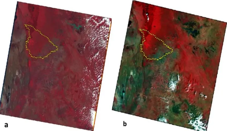
Figure 10 subsets of Landsat images showing the area of interest in false color

a) Landsat 5 TM and b) is a Landsat 8 OLI extracts representing Nairobi River Watershed and displayed in false color infrared (bands 4,3, and 2 for TM and 5,4,3 for OLI displayed as red, green, and blue,

respectively).

Nairobi River Watershed area of interested was masked from both Landsat images as

displayed in Figure 10 a, and b, above. The extracts are also presented in false color infrared to

give vegetation the characteristic reddish appearance for easier identification. Healthy vegetation

the brighter the red appearance, the healthier the vegetation cover. Urban areas and constructed

spaces appear bluish to greyish in this scheme because they reflect less radiation while water

appears dark due to its property of absorbing most of the radiation that falls on it.

3.2.2 LULC Change Detection

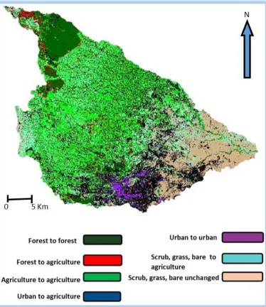
Figure 11 LULC change image

Images a, and b, show the classification of LULC of NRW on 5/1/1986 and 5/1//2015 respectively. The purple

color shows urban, dark green shows forest cover, light green is agricultural area, blue is area under water

and tan is scrub/grass/bare.

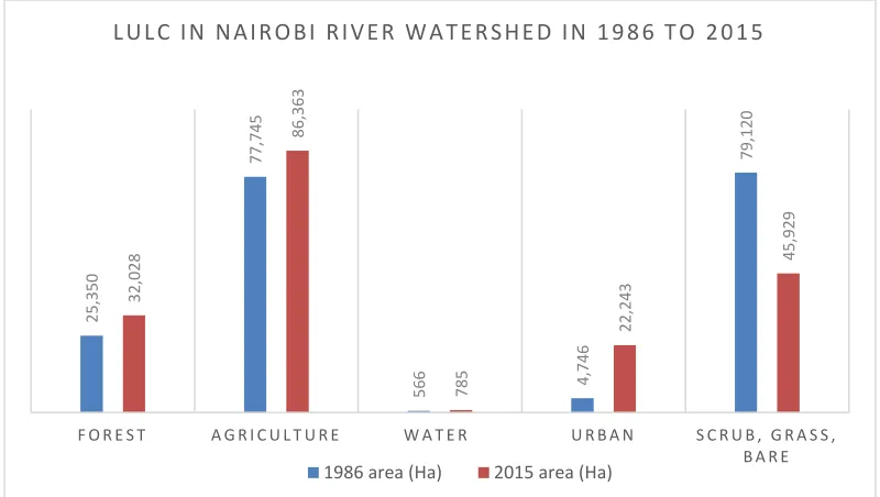
From Figure 11 above and Table 1 below, in 1986, 14% (25,350 ha) of the total land area

of NRW was under forest. In the same year, 0.3% (566 ha) was covered by water, 41% (77,745

Ha) was under agriculture, only 3% (4,746 ha) was urban, and 42% (79,120 ha) was

scrub/grass/bare. In 2015, forest cover increased to about 17% (32,028 ha) of the total land surface

(86,362 ha), urban had 12% (22,243 ha), and the area under scrub/grass/bare shrunk to 25%

(45,929 ha).

Table 1 LULC classification of Nairobi River Watershed in 1986 and 2015

LULC 1986 area

(Ha) 2015 area (Ha) % area 1986 % area 2015

Change (Ha) %

Change

Forest 25,349.70 32,028.20 13.52 17.10 6,678.5 26

Agriculture 77,744.60 86,362.50 41.46 46.10 8,617.9 11

Water 566.46 784.64 0.30 0.42 218.18 39

Urban 4,746.00 22,243.30 2.53 11.87 17,497 369

Scrub/grass/bare 79,119.70 45,928.83 42.19 24.52 - 33,190.87 -42

This Table displays the total area in Ha of each LULC in 1986 and 2015 respectively, their percentage cover and the differences between the two periods in Ha and percentages. The percentage change was computed from the change in Ha divided by the specific LULC in 1986.

Figure 12 LULC of Nairobi River Watershed in 1986 and 2015

25, 350 77, 745 566 4, 746 79, 120 32, 028 86, 363 785 22, 243 45, 929

F O R E S T A G R I C U L T U R E W A T E R U R B A N S C R U B , G R A S S ,

B A R E L U L C I N N A I R O B I R I V E R W A T E R S H E D I N 1 9 8 6 T O 2 0 1 5

During the 30 years’ period, urban development increased by 369% (17,497 ha), and this

was the greatest percentage increase of all LULC. Water class increased by about 39% from 566

Ha to 785 ha. Agriculture class gained coverage by about 11% while the area under forest

increased by 6%. Scrub/grass/bare decreased coverage the most by about 42%.

3.2.2.1 Urbanization, Deforestation, and Agriculture

Figure 13 above presents the trend in Urbanization and deforestation between the year 1986

and 2015. The areas marked with red represent forests that were converted into urban while the

brown color shows areas that were forest and turned into scrub/grass/bare. Cyan symbolizes areas

that were under agriculture and converted into urban areas. Yellow represents scrub/grass/bare

land that turned into urban. Figure 14 below highlights the conversion of other LULC classes into

agriculture whereby the areas shaded with red are portions of forests that were converted into

Figure 14 LULC Change, Agriculture and Deforestation

Table 2 and figure 15 show how LULC gained or lost during the study period. The water

class gained 423 Ha and lost about 204 Ha between 1986 and 2015. The forest class gained cover

by about 14,748 Ha and lost about 8.041 Ha. Agriculture gained about 35,746 Ha and lost about

27,093 Ha during the period under consideration. The urban class had the least loss relative to the

gain, whereby the class lost about 1,944 Ha and gained 19,426 Ha. The scrub/grass/bare class

Table 2 LULC gains and loses between 1986 and 2015

Class Gain Loss Net Change

Forest 14,748 8,041 6,707

Agriculture 35,746 27,093 8,653

Water 423 204 219

Urban 19,426 1,944 17,482

Scrub/grass/bare 12,682 45,753 -33,071

Figure 15 LULC gains and losses between 1986 and 2015

3.3 Geochemistry

3.3.1 Major Elements

The concentration of major oxides, inorganic carbon and sulfur did not change abruptly

along Nairobi River gradient. There was no significant pattern to suggest any increase or decrease

in the intensity of this group as the river flowed through the different LULC classes. However,

there was a weak decreasing trend of Al2O3 down the river gradient (Figure 16 and 17). Table 3

14, 748 35, 746 423 19, 426 12, 682 8, 041 27, 093 204 1, 944 45, 753

F O R E S T A G R I C U L T U R E W A T E R U R B A N S C R U B , G R A S S ,

B A R E L U L C G A I N S A N D L O S E S ( H A ) I N N R W B E T W E E N 1 9 8 6

A N D 2 0 1 5

below presents the distribution of major oxides, inorganic carbon and sulfur down the gradient of

Nairobi River. It is worth noting that the trend of Na2O and K2O down the river gradient followed

an identical pattern. This is because Na and K are both group one (alkali) metals in the periodic

table and therefore they exhibit similar chemical reactions.

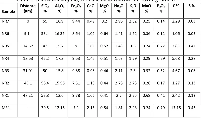
Table 3 Distribution of major elements down Nairobi River gradient Sample Distance (Km) SiO2 %

Al2O3

%

Fe2O3

%

CaO %

MgO %

Na2O

%

K2O

%

MnO %

P2O5

%

C % S %

NR7 0 55 16.9 9.44 0.49 0.2 2.96 2.82 0.25 0.14 2.29 0.03

NR6 9.14 53.4 16.35 8.64 1.01 0.64 1.41 1.62 0.36 0.11 1.06 0.02

NR5 14.67 42 15.7 9 1.61 0.52 1.43 1.6 0.24 0.77 7.81 0.47

NR4 18.63 45.2 17.3 9.63 1.45 0.51 1.63 1.79 0.29 0.59 5.68 0.28

NR3 31.01 50 15.8 9.88 0.98 0.46 2.11 2.3 0.52 0.52 4.67 0.08

NR2 45.1 58.4 15.55 7.51 1.19 0.44 2.78 2.73 0.26 0.17 1.27 0.13

NR1 47.21 57.8 12.6 9.78 1.61 0.41 2.7 2.75 0.68 0.41 2.42 0.12

MR1 - 39.5 12.15 7.1 2.16 0.54 1.81 2.03 0.24 0.79 13.15 0.43

There was a noticeable difference between the concentration of major elements in samples

collected along Nairobi River and the only sample collected in Mathare River (MR). The Mathare

River channel’s sediment recorded the least concentration of SiO4 (39.5%), Al2O3 (12.15%) and

Fe2O3 (7.1%). On the other hand, the Mathare sample recorded the highest values for inorganic

carbon (13.15%) while the highest concentration of carbon in NR was NR5 (7.81%). This elevated

level of inorganic carbon is probably associated with the vegetation characteristics of the

catchment and/or the banks of MR in the higher reaches. CaO was also very high in the MR sample

than any of NR samples.

Figure 16 Distribution of major elements down the river gradient

Figure 17 Distribution of major elements without SiO2

0 10 20 30 40 50 60 70 N R 7 N R 6 N R 5 N R 4 N R 3 N R 2 N R 1 MR1 % co n ce n tra tio n

The Trend of major elements down Nairobi River gradient

SiO2 % Al2O3 % Fe2O3 % CaO % MgO % Na2O % K2O % MnO % P2O5 % C % S % 0 2 4 6 8 10 12 14 16 18 20 N R 7 N R 6 N R 5 N R 4 N R 3 N R 2 N R 1 M R 1 % Co n ce n tr ati o n

T h e Tren d o f Maj o r E l ement s w i t h o u t Si O₂ Do w n Nai ro b i Ri ver G rad i ent

3.3.2 Trace Elements

Trace elements revealed a different pattern, unlike the major elements that had no apparent

change down the river. There was a definite increase in the concentration of trace elements down

the river gradient. The highest concentrations were recorded in samples collected from the urban

class and the concentrations reduced in the samples collected outside the city (see Figure 18 and

Table 4 below). There was an increase in the concentration of all heavy metals considered (Sn, As,

Hg, Sb, Ag, Cu, Ni, and Pb) in NR3 (urban class). MR1 sample was corrected from within the

urban class but from a different river and had the second highest concentration of Cu after NR3.

Lead and antimony recorded the highest intensity at 3400 ppm and 187.5 ppm respectively in NR3.

Antimony increased by more than 100 times and Pb by about 41 times in NR3 than in the sample

with the second highest values.

Table 4 Concentration of heavy metals in ppm SAMPLE

NAME

Distance

(Km)

LULC Sn As Hg Sb Ag Cu Ni Pb

NR7 0 Agriculture 12 3.3 0.044 0.41 0.25 11 11 44

NR6 9.14 Agriculture 7 2.9 0.03 0.22 0.25 10 20 33

NR5 14.67 Agriculture/Urban 8 3.4 0.082 0.77 0.25 34 19 44

NR4 18.63 Agriculture/Urban 10 3.5 0.107 0.77 0.25 38 21 52

NR3 31.01 Urban 80 22.5 0.564 187.5 3.9 87 30 3400

NR2 45.1 Scrub/grass/bare 9 1.9 0.076 0.65 0.5 26 12 60

NR1 47.21 Scrub/grass/bare 19 4.5 0.219 1.85 0.5 34 17 83

MR1 - Urban 9 4.5 0.344 1.52 0.8 66 16 65

Correlation coeff’ 1

0.25 0.18 0.40 0.18 0.26 0.39 0.07 0.19

Correlation coeffi’ 2

0.78 0.80 0.85 0.79 0.79 0.94 0.96 0.79

Figure 18 Distribution of heavy metals

This graph presents the distribution of trace elements down Nairobi River gradient, with lead displayed on secondary axis to the right.

To understand these concentrations better, table 5 below compares the highest, lowest and

the average concentrations from each sample to the USEPA risk based (RB) soil screening levels

(SSL) for the protection of groundwater. Table 5 also shows the detection ratios (DR) of elements

which is the ratio of detected concentration divided by the USEPA soil screening levels. 0 500 1000 1500 2000 2500 3000 3500 4000 0 20 40 60 80 100 120 140 160 180 200

NR7 NR6 NR5 NR4 NR3 NR2 NR1 MR1

Con ce n tra tio n o f P b in p p m Con ce n tra tio n in p p m

Concentration of heavy metals down Nairobi River gradient

Figure 19 LULC and samples collection points

Figure 19 displays a classified Landsat 8 OLI image of Nairobi River Watershed in May 2015, the length of the River sampled and the samples collection points.

A detection ratio (DR) of 22,700 was recorded for lead in NR3 and 220 in the lowest sample

(NR6). As recorded a high DR of 15,000 in NR3 (urban) and a low of 1930 in NR2

(scrub/grass/bare). The highest detection ratio for Sb was 536 from NR3 and the lowest was 0.629

from NR6. Cr recorded a high DR of 9000 and a low of 3000 while Cd had a high DR of 1 and a

low of 0.36. Ni and Cu had high DRs of 115 and 3 respectively and low of 4 and 0.3 respectively.

Sn had the lowest DR of 0.03 for the sample with the highest concentration and a low of 0.002.

The urban class (NR3) recorded all the high DRs while NR6 (agriculture) and NR2

Table 5 Concentration of primary heavy metals in ppm

Element Highest Lowest Average EPA RB SSL Highest DR Lowest

DR

Sn 80 7 19.25 3000 2.67E-02 2.33E-03

As 22.5 2.9 5.81 0.0015 1.50E+04 1.93E+03

Hg 0.564 0.03 0.18 0.018 3.13E+01 1.67E+00

Sb 187.5 0.22 24.21 0.35 5.36E+02 6.29E-01

Ni 30 11 18.25 0.26 1.15E+02 4.23E+01

Pb 3400 33 472.63 0.15 2.27E+04 2.20E+02

Cd 0.75 0.25 0.35 0.69 1.09E+00 3.62E-01

Ce 769 237 444.75 - - -

Cr 90 30 50 0.001 9.00E+03 3.00E+03

Cu 87 10 38.25 28 3.11E+00 3.57E-01

Table 5 shows the concentrations of primary heavy metals in ppm, the EPA RB (Risk Based) SSL (Soil Screening Levels) for the protection of groundwater (https://semspub.epa.gov/work/HQ/197025.pdf) and the detection ratios. The EPA values are given in mg/Kg which is equivalent to ppm (1 mg/Kg = 1 part/million). The table presents the highest recorded concentration, the minimum, the average of all records and the USEPA limits. The table also shows the detection ratios (DR) of the samples with the highest and the lowest concentration.

The highest concentration of heavy metals contamination was observed in the samples from the

urban classes. For instance, tin concentration increased by eight times from 10 ppm in NR4 to

80ppm in NR3. In this section, Pb increased from 52 ppm to 3400 ppm a two order of magnitude

increase or more than 65 times the previous sampled section. The intensity of all the trace elements

increased between NR4 and NR3 by about 1.5 times to 65 times. Figure 20 a, and b, shows the

concentration of elements down the river gradient. Lead increased the most, and therefore it is

plotted separately on a logarithmic scale along the vertical axis in Figure 20b. Similarly, there was

a big decrease in heavy metals’ concentration between NR3 sample and the next (NR2) down the

Figure 20 Concentration of trace elements down the river gradient

Figure 20 a, and b, show an increasing concentration of trace elements down the river gradient. Figure 20 b is on logarithmic scale in the vertical axis because of higher differences in concentration of lead.

The trends in figures 20 a, and b, show an increasing concentration of heavy metals down

the gradient of Nairobi River for most of the trace elements analyzed. These trends suggest a

gradual introduction of heavy metals as the river flow down the gradient. Concentrations of other

elements like As, Hg and Ag were relatively constant down the river except at NR3 sample that

peaked for all elements. There was a significantly high correlation between the concentration of

heavy metals and the distance along the gradient of the river up to and including the urban class.

The concentration reduced considerably after the river passed the urban class. The correlation

coefficient of the levels of Sn, As, Hg, Sb, Ag, Cu, Ni, and Pb and the distance along the river up

to the city ranged between 0.78 and 0.96. However, this correlation coefficient reduced to between

Figure 21 Comparison of concentration of heavy metals to allowable limits

Figure 21 compares the major heavy metals with the EPA RB (Risk Based) SSL (Soil Screening Levels) for the protection of groundwater. It shows the relationship between the highest recorded concentration, the minimum, the average of all records and the EPA limits.

3.3.3 Upper Continental Standardized Spider Diagrams

Spider diagrams were used to compare the geochemistry of NR with the upper continental

crust (UCC) for major and rare earth elements (REE). These diagrams are essential for determining

enrichment and depletion ratios of elements in comparison to the UCC values. Juvenile UCC

ranges were adopted from Condie (1997) because these match well with the geochronology of

Nairobi River watershed’s igneous material which dates to about 5 million years ago.

0.0001 0.001 0.01 0.1 1 10 100 1000

Sn As Hg Sb Ni Pb Cd Ce Cr Cu

D

ET

EC

TIO

N

R

A

TIO

Heavy metal concentration in Nairobi River Sediments vs EPA RB (Risk Based) SSL (Soil Screening Levels) for

the protection of groundwater

Figure 22 Enrichment/depletion of selected elements against the UCC values

Figure 22 shows Spider diagrams displaying the ratios of enrichment/depletion of selected elements in comparison to the juvenile upper continental crust’s values (a) shows the major elements (b) and (c) show rare earth elements and (d) represents Pb distribution.

From Figure 22a above, oxides of Si, Ca and Mg from all the samples exhibited depletion

from that of the juvenile UCC values. Oxides of Al, Na, and K, were just about equal values with

the UCC values, while those of Fe, Mn and, Ti were conspicuously enriched in all the samples.

Phosphate oxides behaved differently whereby in three samples the enrichment factors were about

one while in the rest of the samples, concentration rose to a maximum of about five times more

than that of the juvenile UCC. The three samples that exhibited equal concentration of P2O5 to that

from NR2 (scrub/grass/bare). MnO also behaved like P2O5 in that there was a big disparity among

samples ranging from an enrichment factor of 2.4 to 6.8. This inconsistency suggests

anthropogenic introduction of Mn and P along the river gradient.

Figures 22 b, and c, present a mixture of light rare earth elements (LREE), heavy rare earth

elements (HREE) and other trace elements normalized with the juvenile UCC values. Different

elements scored differently in which a good number exhibited depletion. Rb remained about the

same concentration to the juvenile UCC while several other elements were significantly enriched.

Elements that exhibited depletion included Ni, Ba, Co, Sr, V, and Sc. Arsenic had similar

characteristics of depletion except for NR5 sample which had an enrichment factor of 4.5. Cu

had a similar trend also, in which two samples were significantly depleted, four showed almost

similar concentrations with the juvenile UCC values, while two were enriched from the juvenile

UCC values. The rest of the elements in figures 22 b and c, showed varying factors of enrichment

ranging from about 2 to 15 times. Er recorded the highest enrichment factor of about 15.2 in NR7

and the lowest of about 7.4 in NR2. Cerium had enrichment factors of between 3 at NR 2 and 12

at NR6, while La recorded enrichment factors of between 3 and 10 with the NR6 sample showing

the highest enrichment. Lu was highly enriched at NR7 where it recorded an enrichment factor of

about eight times and the least enrichment of three times in NR2. Nd was highly enriched in NR 6

with enrichment factors of between 2.5 and 6.7. Sm and Tb were highly enriched in NR7 and NR6

with enrichment factors of 6.5 and 6 respectively, and lowest in NR2 with enrichment factors of

3.2 and 2.9 respectively. Th and Zr were highest enriched in NR7 with enrichment factors of 4.2

and 9.7 respectively and lowest enriched in NR1 with enrichment factors of 1.68 and 3.98

respectively. Yb and Sn exhibited a wide range of enrichment factors down the river gradient with